物体检测算法通常在输入图像中对大量区域进行采样，确定这些区域是否包含感兴趣的对象，并调整区域的边缘，以便更准确地预测目标的真实边界框。不同的模型可能使用不同的区域抽样方法。这里，我们介绍了一种这样的方法:它以每个像素为中心生成多个不同大小和宽高比的边框。这些边界框称为Anchor。我们将在下面几节中练习基于Anchor的对象检测。

首先，导入本节所需的包或模块。这里，我们修改了PyTorch的打印精度。因为打印张量实际上调用了PyTorch的打印函数，所以本节打印的张量中的浮点数更简洁。

%matplotlib inline
from d2l import torch as d2l
import torch

torch.set_printoptions(2)

Generating Multiple Anchor Boxes

假设输入图像的高度为 $h$，宽度为 $w$。我们生成以图像每个像素为中心的不同形状的Anchor。假设尺寸 $s \in (0, 1]$，宽高比 $r > 0$， Anchor框的宽度和高度分别是 $ws\sqrt{r}$ 和 $hs / \sqrt{r}$。当给定中心位置时，确定一个已知宽度和高度的Anchor框。

下面我们设置一组尺寸$s_1, …, s_n$ 和一组宽高比 $r_1, …, r_m$。如果我们使用所有大小和宽高比的组合，以每个像素为中心，输入图像将有 $whnm$ 个 Anchor 框。尽管这些 Anchor 框可以覆盖所有的ground-truth边界框，但计算复杂度往往过高。因此，我们通常只对包含尺寸为 $s1$ 或宽高比为$r1$ 的组合感兴趣，也就是说：

\[(s_1, r_1), (s_1, r_2), ..., (s_1, r_m), (s_2, r_1), (s_3, r_1), ..., (s_n, r_1) \tag{1}\]

即，以同一像素为中心的 Anchor 框个数为 $n + m - 1$。对于整个输入图像，我们将生成总共 $wh(n + m - 1)$ 个Anchor框。

上述产生Anchor框的方式由 multibox_prior 函数实现。我们指定输入、一组大小和一组宽高比，这个函数将返回所有输入的 Anchor 框。

#@save
def multibox_prior(data, sizes, ratios):
    """
    args: 
        data : 图像
        sizes : 尺寸集
        ratios : 宽高比集
     
    return: 
        output(tensor) : 用在dataloader中可将anchor组成batch 
    """

    #--- tensor的后两维就是图像的高和宽 ---
    in_height, in_width = data.shape[-2:]

    #--- device: cpu or cuda ---
    #--- num_sizes: 就是尺寸的个数 n ---
    #--- num_ratios: 就是宽高比的个数 m---
    device, num_sizes, num_ratios = data.device, len(sizes), len(ratios)

    #--- 每个像素有 (n + m - 1) 个anchor框 ---
    boxes_per_pixel = (num_sizes + num_ratios - 1)

    size_tensor = torch.tensor(sizes, device=device)
    ratio_tensor = torch.tensor(ratios, device=device)

    #--- offset 用于将anchor移动到每个像素的中心 ---
    #--- steps_h, steps_w 是归一化的系数，用于将图像的宽高归一化到0到1之间---
    offset_h, offset_w = 0.5, 0.5
    steps_h = 1.0 / in_height
    steps_w = 1.0 / in_width

    #--- 假设图像为 256 x 512 ---
    #--- 首先将 x 轴 和 y 轴都加0.5， 使得anchor位于每个像素的中心 --- 
    #--- 再将宽高进行归一化 --- 
    center_h = (torch.arange(in_height, device=device) + offset_h) * steps_h
    center_w = (torch.arange(in_width, device=device) + offset_w)  * steps_w

    #--- h:(0.5, 1.5, ..., 255.5) -> 归一化 ---
    #--- w:(0.5, 1.5, ..., 511.5) -> 归一化 ---
    #--- meshgrid的返回值： ---
    #--- shift_y:  (0.5, 0.5, ..., 0.5) ---
    #---           (1.5, 1.5, ..., 1.5) ---
    #---                      ...         ---
    #---           (255.5, 255.5, ..., 255.5) ---
    #--- 共256行， 共512列， 数值为未归一化时的数值 ---
    #--- shift_x:  (0.5, 1.5, ..., 511.5) ---
    #---           (0.5, 1.5, ..., 511.5) ---
    #---                      ...         ---
    #---           (0.5, 1.5, ..., 511.5) ---
    #--- 共256行， 共512列, 数值为未归一化时的数值 ---
    shift_y, shift_x = torch.meshgrid(center_h, center_w)
    #--- shift_y, shift_x shape: (256 x 512) ---
    shift_y, shift_x = shift_y.reshape(-1), shift_x.reshape(-1)


    #--- w_anchor = w * s * sqrt{r} ---
    #--- 因为已经做过归一化了， 所以这里 w 就是 1 ---
    #--- 由于ssd最初是为方形图像（300x300）开发的，因此 in_height / in_width 用于处理矩形输入---
    w = torch.cat((size_tensor * torch.sqrt(ratio_tensor[0]), sizes[0] * torch.sqrt(ratio_tensor[1:]))) * in_height / in_width
    h = torch.cat((size_tensor / torch.sqrt(ratio_tensor[0]), sizes[0] / torch.sqrt(ratio_tensor[1:])))

    
    #--- w_anchor = w * s * sqrt{r} 和 h_anchor = h * s / sqrt{r} 都是正数 ---
    #--- 为了让anchor可以上下左右移动， 需要对 w_anchor 和 h_anchor 除以2再取正负 ---
    anchor_manipulations = torch.stack((-w, -h, w, h)).T.repeat(in_height * in_width, 1) / 2

    #--- 四个轴分别对应每个 anchor 的 left, bottom, right, top ---
    #--- 形状： (h * w * (n + m - 1), 4) ---
    out_grid = torch.stack([shift_x, shift_y, shift_x, shift_y], dim=1).repeat_interleave(boxes_per_pixel, dim = 0)


    output = out_grid + anchor_manipulations

    #--- 将 anchors组成batch  ---
    return output.unsqueeze(0)

w = torch.cat((size_tensor * torch.sqrt(ratio_tensor[0]),
                   sizes[0] * torch.sqrt(ratio_tensor[1:])))\
                   * in_height / in_width

为什么这里要乘以 in_height / in_width ?

A：由于ssd最初是为方形图像（300x300）开发的，因此 in_height / in_width 用于处理矩形输入。

可以看出，返回的 Anchor 框变量y的形状为 (batch size，number of anchor boxes，4)。

img = d2l.plt.imread('../img/catdog.jpg')
h, w = img.shape[0:2]

print(h, w)
X = torch.rand(size=(1, 3, h, w))  # Construct input data
Y = multibox_prior(X, sizes=[0.75, 0.5, 0.25], ratios=[1, 2, 0.5])
Y.shape

输出：

561 728

torch.Size([1, 2042040, 4])

将Anchor框的变量 Y 的形状改变为(图像高度，图像宽度，以同一像素为中心的Anchor框数量，4)后，我们可以得到以指定像素为中心的所有Anchor框。在下面的例子中，我们访问第一个以(250,250)为中心的Anchor框。它有四个元素:位于Anchor框左上角的x、y轴坐标和位于Anchor框右下角的x、y轴坐标。x 轴和 y 轴的坐标值分别除以图像的宽度和高度，取值范围为 $0 \thicksim 1$。

boxes = Y.reshape(h, w, 5, 4)
boxes[250, 250, 0, :]

输出：

tensor([0.06, 0.07, 0.63, 0.82])

为了描述图像中以一个像素为中心的所有Anchor框，我们首先定义 show_bboxes 函数来在图像上绘制多个边界框。

#@save
def show_bboxes(axes, bboxes, labels=None, colors=None):
    """Show bounding boxes."""
    def _make_list(obj, default_values=None):
        if obj is None:
            obj = default_values
        elif not isinstance(obj, (list, tuple)):
            obj = [obj]
        return obj

    labels = _make_list(labels)
    colors = _make_list(colors, ['b', 'g', 'r', 'm', 'c'])
    for i, bbox in enumerate(bboxes):
        color = colors[i % len(colors)]
        rect = d2l.bbox_to_rect(bbox.detach().numpy(), color)
        axes.add_patch(rect)
        if labels and len(labels) > i:
            text_color = 'k' if color == 'w' else 'w'
            axes.text(rect.xy[0],
                      rect.xy[1],
                      labels[i],
                      va='center',
                      ha='center',
                      fontsize=9,
                      color=text_color,
                      bbox=dict(facecolor=color, lw=0))

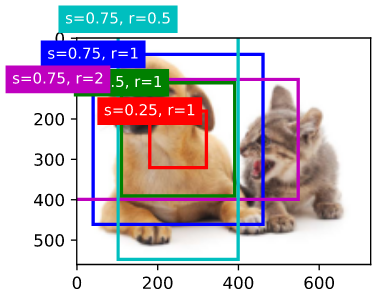
正如我们刚才看到的，变量框中的 $x$ 轴和 $y$ 轴的坐标值分别除以图像的宽度和高度。在绘制图像时，我们需要恢复Anchor框的原始坐标值，因此定义变量 bbox_scale。现在，我们可以在图像中以(250,250)为中心绘制所有Anchor框。如你所见，大小为0.75、宽高比为1的蓝色Anchor框很好地覆盖了图像中的狗。

d2l.set_figsize()
bbox_scale = torch.tensor((w, h, w, h))
fig = d2l.plt.imshow(img)
show_bboxes(fig.axes, boxes[250, 250, :, :] * bbox_scale,
            ['s=0.75, r=1', 's=0.5, r=1', 's=0.25, r=1', 's=0.75, r=2',
             's=0.75, r=0.5'])

Intersection over Union

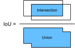
我们刚刚提到，Anchor框很好地覆盖了图像中的狗。如果目标的真实边界框是已知的，怎么能很好地在这里量化？一种直观的方法是测量Anchor框与真实边界框之间的相似性。我们知道，Jaccard指标可以度量两个集合之间的相似性。给定集合 $A$ 和 $B$，它们的Jaccard指标是它们交集的大小除以它们并集的大小。

\[J(A, B) = \frac{\mid A \cap B \mid}{\mid A \cup B \mid} \tag{2}\]

事实上，我们可以把边界框的像素区域看作是像素的集合。这样，我们就可以通过两个边界框的像素集的Jaccard索引来度量这两个边界框的相似性。当我们测量两个边界框的相似性时，我们通常将Jaccard指标称为交并比(intersection over union, IoU)，它是两个边界框相交面积与并集面积的比值，如图13.4.1所示。IoU的取值范围为 $0 \thicksim 1$, 0表示两个边界框之间没有重叠像素，1表示两个边界框相等。

Fig. 13.4.1 IoU是两个边界框的相交面积与合并面积的比值。

在本节的其余部分中，我们将使用IoU来度量Anchor框和ground-truth边界框以及不同Anchor框之间的相似性。

#@save
def box_iou(boxes1, boxes2):
    #--- 计算形状为(N, 4) 和 (M, 4)的boxes的交并比 ---
    #--- 计算面积 ---
    box_area = lambda boxes: ((boxes[:, 2] - boxes[:, 0]) * boxes[:, 3] - boxes[:, 1])

    area1 = box_area(boxes1)
    area2 = box_area(boxes2)

    #--- None用于增加维度， boxes1中的每个元素都要和boxes2中的元素进行运算 ---
    #--- 比如 [[1] ---
    #---      [2]] ---
    #--- 和 [3, 4] 进行加法运算 ---
    #--- 得到 [[4], [5]  ---
    #---      [5], [6]] ---
    lt = torch.max(boxes1[:, None, :2], boxes2[:, :2]) # [N, M, 2]
    rb = torch.min(boxes1[:, None, 2:], boxes2[:, 2:]) # [N, M, 2]
    wh = (rb - lt).clamp(min=0) #[N, M, 2]
    inter = wh[:, :, 0] * wh[:, :, 1] #[N, M]
    unioun = area1[:, None] + area2 - inter
    
    return inter / unioun

它的输出为 (N, M)， N为 Anchor Box 个数， M 为 Ground-truth Box 个数。

Labeling Training Set Anchor Boxes

在训练集中，我们将每个Anchor框作为一个训练示例。为了训练目标检测模型，我们需要为每个Anchir框标记两种类型的标签:一是Anchor框中包含的目标类别(category)，二是ground-truth边界框相对于Anchor框的偏移量(offset)。在目标检测中,我们首先生成多个Anchor框, 预测每个Anchor框的category和offset,根据预测的offset调整Anchor框位置得到用于预测的边界框,最后过滤预测边界框, 输出需要的边界框。

我们知道，在目标检测训练集中，每一幅图像都有标记ground-truth边界框的位置和包含的目标类别。Anchor框生成后，我们主要根据与Anchor框相似的ground-truth边界框的位置和category信息对Anchor框进行标注。那么我们如何将ground-truth边界框分配到相似的Anchor框呢？

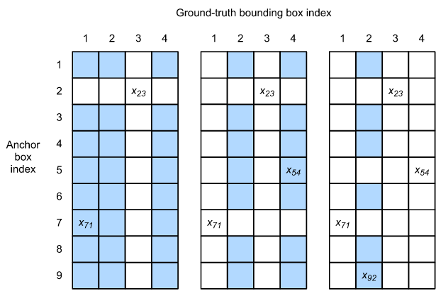
假设在图像中的Anchor框是$A_1, A_2, …, A_{n_a}$以及ground-truth框是$B_1, B_2, …, B_{n_b}$，并且$n_a > n_b$。定义矩阵 $X \in R^{n_a \times n_b}$, 其中第 $i$ 行和第 $j$ 列的$x_{ij}$是Anchor框 $A_i$ 和 ground-truth 边界框 $B_j$的交并比。首先，我们找到矩阵 $X$ 中最大的元素，并记录该元素的行索引和列索引为 $i_1$, $j_1$。我们将ground-truth边界框 $B_{j_1}$分配给Anchor框$A_{i_1}$。显然，Anchor框 $A_{i_1}$ 与 ground-truth 边界框 $B_{j_1}$ 在所有Anchor框和 ground-truth 边界框对中相似性最高。接下来，丢弃矩阵 $X$ 中第$i_1$ 行和第 $j_1$ 列中的所有元素。找到矩阵 $X$ 中剩余的最大元素，并记录该元素的行索引和列索引为 $i_2$, $j_2$。我们将ground-truth边界框 $B_{j_2}$ 分配给 Anchor框 $A_{i_2}$ ，然后丢弃矩阵 $X$ 中第 $i_2$ 行和 $j_2$ 列中的所有元素。此时，矩阵 $X$ 中有两行和两列的元素已经被丢弃。

我们继续，直到丢弃矩阵 $X$ 中 $n_b$ 列中的所有元素。此时，我们已经为 $n_b$ 个Anchor框中的每个Anchor框分配了一个ground-truth边界框。接下来，我们遍历剩下的 $n_a - n_b$ Anchor框。给定Anchor框 $A_i$，根据矩阵 $X$ 的第 $i$ 行，找到 $Ai$ 交并比最大的边界框 $B_j$，当交并比大于预定阈值时，才将 ground-truth 边界框 $B_j$ 赋给Anchor框 $A_i$。

如图13.4.2(左)所示，假设矩阵 $X$ 的最大值为 $x_{23}$，则我们将 ground-truth 边界框 $B_3$ 赋值给Anchor框 $A_2$。然后，我们丢弃矩阵第2行和第3列的所有元素，找到剩余阴影区域中最大的元素 $x_{71}$，并将ground-truth边界框 $B_1$ 赋值给Anchor框 $A_7$。然后，如图13.4.2(中)所示，去掉矩阵第7行、第1列的所有元素，找到剩余阴影区域最大的元素 $x_{54}$ ，将ground-truth边界框 $B_4$ 赋值给Anchor框 $A_5$。最后，如图13.4.2(右)所示，去掉矩阵第5行、第4列的所有元素，找到剩余阴影区域最大的元素 $x_{92}$，将 ground-truth 边界框 $B_2$ 赋值给Anchor框 $A_9$。然后，我们只需要遍历剩下的Anchor框 $A_1$, $A_3$, $A_4$, $A_6$, $A_8$，并根据阈值决定是否为剩下的Anchor框分配ground-truth边界框。

Fig. 13.4.2 将ground-truth边界框分配给Anchor框。

#@save
def match_anchor_to_bbox(ground_truth, anchors, device, iou_threshold=0.5):
    #--- num_anchors: n_{a} ---
    #--- num_gt_boxes: n_{b} ---
    num_anchors, num_gt_boxes = anchors.shape[0], ground_truth.shape[0]

    #--- 输出为 (N, M), N = n_a, M = n_b ---
    jaccard = box_iou(anchors, ground_truth)

    #--- 制造一张哈希表， 用于映射anchor和bbox的关系 ---
    #--- key: anc_i, value: box_j ---
    anchors_bbox_map = torch.full((num_anchors, ), -1, dtype=torch.long, device=device)

    #--- box_iou 返回的就是我用用于筛选 anchor 和 gt_box 的表 ---
    #--- 找到每一行中最大交并比最大的 gt_box 和 anchor， 返回它们的索引(列号) ---
    max_iou, indices = torch.max(jaccard, dim=1)

    #--- 找到交并比大于阈值的anchor索引 ---
    anc_i  = torch.nonzero(max_iou >= 0.5).reshape(-1)
    #--- 找到交并比大于阈值的box索引 ---
    box_j = indices[max_iou >= 0.5]

    #--- 删去这些anchor和box所在的行和列 ---
    col_discard = torch.full((num_anchors, ), -1)
    row_discard = torch.full((num_gt_boxes, ), -1)

    for _ in range(num_gt_boxes):
        max_idx = torch.argmax(jaccard)
        box_idx = (max_idx % num_gt_boxes).long()
        anc_idx = (max_idx / num_gt_boxes).long()
        anchors_bbox_map[anc_idx] = box_idx
        jaccard[:, box_idx] = col_discard
        jaccard[anc_idx, :] = row_discard

    return anchors_bbox_map

接下来我们标记 Anchor 框的类别和偏移量。如果 Anchor框 A 被指定为 ground-truth bbox 框 B，则Anchor框A的类别为B的类别。根据 B和 A 中心坐标的相对位置以及两个框的相对大小设置Anchor框A的偏移量。由于数据集中不同框的位置和大小可能不同，这些相对位置和相对大小通常需要一些特殊的变换，以使偏移量分布更均匀，更容易拟合。设Anchor框 A 及其指定的ground-truth bbox框B的中心坐标为 $(x_a, y_a)$，$(x_b, y_b)$， A 和 B 的宽度分别为 $w_a, w_b$，高度分别为 $h_a, h_b$。在这种情况下，一种常见的技术是将$A$ 的偏移量标记为

\[(\frac{\frac{x_b - x_a}{w_a} - \mu_x}{\sigma_x}, \frac{\frac{y_b - y_a}{h_a} - \mu_y}{\sigma_y}, \frac{log \frac{w_b}{w_a} - \mu_w}{\sigma_w}, \frac{log\frac{h_b}{h_a} - \mu_h}{\sigma_h})\]

这些常量的默认值为 $\mu_x = \mu_y = \mu_w = \mu_h = 0, \sigma_x = \sigma_y = 0.1, \sigma_w = \sigma_h = 0.2$。这个变换在下面的 offset_boxes 函数中实现。如果Anchor框没有被指定为ground-truth边界框，我们只需要将Anchor框的类别设置为background。分类为背景的Anchor 框通常被称为负Anchor框，其余的被称为正Anchor框。

def offset_boxes(anchors, assigned_bb, eps=1e-6):
    c_anc = d2l.box_corner_to_center(anchors)
    c_assigned_bb = d2l.box_corner_to_center(assigned_bb)

    #--- 对 anchor 和 box 进行变换， 除以0.1等于乘以10 ---
    offset_xy = 10 * (c_assigned_bb[:, :2] - c_anc[:, :2]) / c_anc[:, 2:]
    offset_wh = 5 * torch.log(eps + c_assigned_bb[:, 2:] / c_anc[:, 2:] )

    #--- offset.shape: (num of anchors, 4) ---
    offset = torch.cat([offset_xy, offset_wh], axis=1)
    return offset



def multibox_target(anchors, labels):
    batch_size, anchors = labels.shape[0], anchors.squeeze(0)
    batch_offset, batch_mask, batch_class_labels = [], [], []
    device, num_anchors = anchors.device, anchors.shape[0]
    for i in range(batch_size):

        #--- labels: (batch, num_gt_box, 5) ---
        label = labels[i, :, :]

        
        #--- 这里已经将anchor筛选过一轮了 ---
        anchors_bbox_map = match_anchor_to_bbox(label[:, 1:], anchors, device=device)

        #--- mask变量中的元素与每个Anchor框的四个偏移值一一对应 ---
        #--- 通过乘以元素，mask变量中的0可以在计算目标函数之前过滤掉负的类偏移量 ---
        bbox_mask = ((anchors_bbox_map >= 0).float().unsqueeze(-1)).repeat(1, 4)
        class_labels = torch.zeros(num_anchors, dtype=torch.long, device=device)
        assigned_bb = torch.zeros((num_anchors, 4), dtype=torch.float32, device=device)

        indices_true = torch.nonzero(anchors_bbox_map >= 0).reshape(-1)
        bb_idx = anchors_bbox_map[indices_true]

        #--- 标签种类 + 1， 0为背景 ---
        class_labels[indices_true] = label[bb_idx, 0].long() + 1
        assigned_bb[indices_true] = label[bb_idx, 1:]

        offset = offset_boxes(anchors, assigned_bb) * bbox_mask

        #--- offset.reshape(-1): num of anchors x 4 ---
        batch_offset.append(offset.reshape(-1))
        #--- bbox_mask.reshape(-1): numof anchors x 4 ---
        batch_mask.append(bbox_mask.reshape(-1))
        #--- class_labels: num of anchors ---
        batch_class_labels.append(class_labels)


    bbox_offset = torch.stack(batch_offset)
    bbox_mask = torch.stack(batch_mask)
    class_labels = torch.stack(batch_class_labels)

    return (bbox_offset, bbox_mask, class_labels)

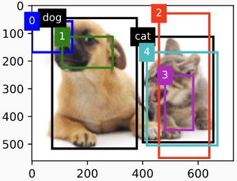
下面我们将演示一个详细的示例。我们为读取的图片中的猫和狗定义 ground-truth bbox，第一个要素是类别(猫为1，狗为0)和剩下的四个要素是 $x, y$ 轴的左上角坐标和 $x, y$ 轴的右下角坐标(0和1之间的值范围)。这里，我们构造了5个Anchor框，分别用左上角和右下角的坐标进行标记，分别记录为 $A_0、、A_4$ (程序中的索引从0开始)。首先，在图像中绘制这些Anchor框和ground-truth边界框的位置。

ground_truth = torch.tensor([[0, 0.1, 0.08, 0.52, 0.92],
                         [1, 0.55, 0.2, 0.9, 0.88]])
anchors = torch.tensor([[0, 0.1, 0.2, 0.3], [0.15, 0.2, 0.4, 0.4],
                    [0.63, 0.05, 0.88, 0.98], [0.66, 0.45, 0.8, 0.8],
                    [0.57, 0.3, 0.92, 0.9]])

fig = d2l.plt.imshow(img)
show_bboxes(fig.axes, ground_truth[:, 1:] * bbox_scale, ['dog', 'cat'], 'k')
show_bboxes(fig.axes, anchors * bbox_scale, ['0', '1', '2', '3', '4'])

我们可以使用 multibox_target 函数为 Anchor框标记类别和偏移量。这个函数将背景类别设置为0，并将目标类别的整数索引从加1(1代表狗，2代表猫)。

我们使用 unsqueeze 函数给 anchor框和 ground-truth bbox 增加维度，并且构造一个随机预测结果，它形状为 (batch_size, number of categories including background, number of anchor boxes) 。

labels = multibox_target(anchors.unsqueeze(dim=0),
                         ground_truth.unsqueeze(dim=0))

返回的结果中有三项，它们都是张量格式。第三项表示标记为Anchor框的类别。

labels[2]

tensor([[0, 1, 2, 0, 2]])

我们根据图像中Anchor框和ground-truth bbox的位置来分析这些已标记的类别。首先，在所有Anchor和ground-truth bbox对中，Anchor框 $A_4$ 对猫的ground-truth 边界框的IoU最大，因此Anchor $A_4$ 的类别被标记为猫。不考虑猫的真实边界框和Anchor边界框 $A_4$，在剩余的Anchor和ground-truth边界框对，狗的真实边界框和Anchor框 $A_1$具有最大交并比，所以Anchor框 $A_1$ 的类别是狗。接下来，遍历其余三个未标记的Anchor框。Anchor框 $A_0$ 具有最大交并比的真实边界框的种类是狗，但是交并比小于阈值(默认为0.5)，因此种类被标记为背景； Anchor框 $A_2$ 具有最大交并比的真实边界框的种类是猫，并且交并比大于阈值，因此种类被标记为猫； Anchor框 $A_3$ 具有最大交并比的真实边界框的种类是猫，但是交并比小于阈值(默认为0.5)，因此种类被标记为背景；

返回值的第二项是一个mask变量，它的形状是 (batch size, four times the number of anchor boxes)。 mask变量中的元素与每个Anchor框的四个偏移值一一对应。因为我们不关心背景检测，负类的偏移量不应该影响目标函数。通过乘以元素，mask变量中的0可以在计算目标函数之前过滤掉负类的偏移量。

labels[1]


tensor([[0., 0., 0., 0., 1., 1., 1., 1., 1., 1., 1., 1., 0., 0., 0., 0., 1., 1.,
         1., 1.]])

返回的第一项是为每个Anchor框标记的四个偏移值，负类Anchor框的偏移值标记为0。

labels[0]

tensor([[-0.00e+00, -0.00e+00, -0.00e+00, -0.00e+00,  1.40e+00,  1.00e+01,
          2.59e+00,  7.18e+00, -1.20e+00,  2.69e-01,  1.68e+00, -1.57e+00,
         -0.00e+00, -0.00e+00, -0.00e+00, -0.00e+00, -5.71e-01, -1.00e+00,
          4.17e-06,  6.26e-01]])

Bounding Boxes for Prediction

在模型预测阶段，我们首先为图像生成多个Anchor框，然后对这些Anchor框逐个预测类别和偏移量。然后，根据Anchor框及其预测偏移量得到预测边界框。

下面我们实现函数 offset_inverse，它接受 anchors 和offset predictions作为输入，并应用逆偏移量变换来返回预测的边框坐标。

#@save
def offset_inverse(anchors, offset_preds):
    c_anc = d2l.box_corner_to_center(anchors)
    c_pred_bb_xy = (offset_preds[:, :2] * c_anc[:, 2:] / 10) + c_anc[:, :2]
    c_pred_bb_wh = torch.exp(offset_preds[:, 2:] / 5) * c_anc[:, 2:]
    c_pred_bb = torch.cat((c_pred_bb_xy, c_pred_bb_wh), axis=1)
    predicted_bb = d2l.box_center_to_corner(c_pred_bb)
    return predicted_bb

当有许多Anchor框时，同一个目标可能会输出许多类似的预测边界框。为了简化结果，我们可以删除类似的预测框。一种常用的方法称为非极大抑制(NMS)。

让我们来看看NMS是如何工作的。对于一个预测的边界框 $B$，模型计算每个类别的预测概率。假设最大的预测概率是 $p$，这个概率对应的类别就是 $B$ 的预测类别。在同一幅图像上，根据置信度从高到低对除背景外以外预测类别的预测边框进行排序，得到列表 $L$。从 $L$ 中选择置信度最高的预测边界框 $B_1$ 作为基线，计算$B_1$与其它边界框的交并比，从 $L$ 中删除所有与 $B_1$ 交并比小于某一阈值非基准预测边界框。这里的阈值是一个预置的超参数。此时，$L$ 保留了置信度最高的预测边界框，并删除了其他类似的预测边界框。接下来，选择 $L$ 中置信度第二高的预测边界框 $B_2$ 作为基线，计算$B_2$与其它边界框的交并比，删除 $L$ 中所有与 $B_2$ 交并比小于某一阈值的所有非基准预测边界框。重复这个过程，直到 $L$ 中的所有预测框都被用作基线。此时，$L$ 中任何一对预测框的IoU都大于阈值。最后，将所有预测框输出到列表 $L$ 中。

#@save
def nms(boxes, scores, iou_threshold):
    # sorting scores by the descending order and return their indices
    B = torch.argsort(scores, dim=-1, descending=True)
    keep = []  # boxes indices that will be kept
    while B.numel() > 0:
        i = B[0]
        keep.append(i)
        if B.numel() == 1: break
        # 计算置信度最高的box 和 其余box 的 IoU
        # shape: (M, N) -> M * N
        iou = box_iou(boxes[i, :].reshape(-1, 4),
                      boxes[B[1:], :].reshape(-1, 4)).reshape(-1)

        print(iou.shape)

        inds = torch.nonzero(iou <= iou_threshold).reshape(-1)
        print(inds)
        B = B[inds + 1]
    return torch.tensor(keep, device=boxes.device)

#@save
def multibox_detection(cls_probs, offset_preds, anchors, nms_threshold=0.5,
                       pos_threshold=0.00999999978):
    device, batch_size = cls_probs.device, cls_probs.shape[0]
    print("batch_size: ", batch_size)
    # 每次只能输入batch 1
    anchors = anchors.squeeze(0)
    num_classes, num_anchors = cls_probs.shape[1], cls_probs.shape[2]
    out = []
    for i in range(batch_size):
        # 挨个把类的概率 和 预测的偏移量 拿出来
        cls_prob, offset_pred = cls_probs[i], offset_preds[i].reshape(-1, 4)
        # 求anchor框是猫还是狗， 返回元组([value1, valu2, ...]， [index1, index2, ...])
        conf, class_id = torch.max(cls_prob[1:], 0)
        # 根据anchor框和预测的偏移量 得到 预测的边界框
        predicted_bb = offset_inverse(anchors, offset_pred)
        # NMS之后保留下的预测框， 它是一个索引组成的列表
        keep = nms(predicted_bb, conf, 0.5)

        # Find all non_keep indices and set the class_id to background
        all_idx = torch.arange(num_anchors, dtype=torch.long, device=device)
        combined = torch.cat((keep, all_idx))
        uniques, counts = combined.unique(return_counts=True)
        non_keep = uniques[counts == 1]
        all_id_sorted = torch.cat((keep, non_keep))
        class_id[non_keep] = -1
        # 将class_id 调整为keep在前，non_keep在后的顺序
        class_id = class_id[all_id_sorted]
        conf, predicted_bb = conf[all_id_sorted], predicted_bb[all_id_sorted]
        # threshold to be a positive prediction
        below_min_idx = (conf < pos_threshold)
        class_id[below_min_idx] = -1
        conf[below_min_idx] = 1 - conf[below_min_idx]
        pred_info = torch.cat((class_id.unsqueeze(1),
                               conf.unsqueeze(1),
                               predicted_bb), dim=1)
        out.append(pred_info)
    return torch.stack(out)

接下来，我们将看一个详细的示例。首先，构建四个Anchor框。为了简单起见，我们假设预测偏移量都为0。这意味着预测框就是Anchor框。最后，我们为每个类别构造一个预测概率。

anchors = torch.tensor([[0.1, 0.08, 0.52, 0.92], [0.08, 0.2, 0.56, 0.95],
                        [0.15, 0.3, 0.62, 0.91], [0.55, 0.2, 0.9, 0.88]])
offset_preds = torch.tensor([0] * anchors.numel())
cls_probs = torch.tensor([
    [0] * 4,  # Predicted probability for background
    [0.9, 0.8, 0.7, 0.1],  # Predicted probability for dog
    [0.1, 0.2, 0.3, 0.9]
])  # Predicted probability for cat

在图像上打印预测边框及其置信度。

fig = d2l.plt.imshow(img)
show_bboxes(fig.axes, anchors * bbox_scale,
            ['dog=0.9', 'dog=0.8', 'dog=0.7', 'cat=0.9'])

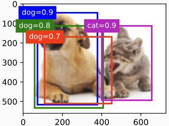
我们使用 multibox_detection 函数进行 NMS，将阈值设置为0.5。这样就给张量输入增加了一个维数。可以看到，返回结果的形状为 (batch size, number of anchor boxes, 6)。每行的6个元素表示同一个预测框的输出信息。第一个元素是预测的类别索引，它从0开始(0是dog, 1是cat)。-1 表示背景或者用NMS删除。第二个元素是预测边界框的置信度。其余四个元素是预测框左上角的 $x、y$ 轴坐标和右下角的 $x、y$轴坐标(取值范围在0到1之间)。

output = multibox_detection(cls_probs.unsqueeze(dim=0),
                            offset_preds.unsqueeze(dim=0),
                            anchors.unsqueeze(dim=0),
                            nms_threshold=0.5)
output

tensor([[[ 0.00, 0.90, 0.10, 0.08, 0.52, 0.92], [ 1.00, 0.90, 0.55, 0.20, 0.90, 0.88], [-1.00, 0.80, 0.08, 0.20, 0.56, 0.95], [-1.00, 0.70, 0.15, 0.30, 0.62, 0.91]]])

我们去掉类别-1的预测框，并将NMS保留的结果可视化。

fig = d2l.plt.imshow(img)
for i in output[0].detach().numpy():
    if i[0] == -1:
        continue
    label = ('dog=', 'cat=')[int(i[0])] + str(i[1])
    show_bboxes(fig.axes, [torch.tensor(i[2:]) * bbox_scale], label)

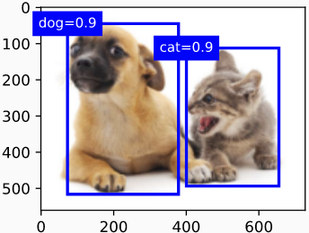
在实践中，我们可以在执行NMS之前删除具有较低置信度的预测框，从而减少NMS的计算量。我们还可以过滤NMS的输出，例如, 只保留具有较高置信度的结果作为最终输出。

Summary

我们生成了多个以每个像素为中心的大小和宽高比不同的Anchor框。
IoU，也称为Jaccard指数，衡量两个边界框的相似性。它是两个边界框的相交面积与联合面积之比。
在训练集中，我们为每个 Anchor 框标记两种类型的标签:一种是 Anchor 框中包含的目标类别，另一种是ground-truth边界框相对于Anchor框的偏移量。
在进行预测时，我们可以使用非极大值抑制(non-maximum suppression, NMS)去除相似的预测框，从而简化结果。

Exercises

改变 multibox_prior 函数中的 sizes 和 ratios，并观察生成的Anchor框的变化。
构建两个IoU为0.5的边界框，并观察它们的重合情况。
通过标记本节定义的Anchor框偏移量来验证offset label[0]的输出(常量是默认值)
修改 “Labeling Training Set Anchor Boxes” 和 “Output Bounding Boxes for Prediction” 部分中的 Anchor变量。结果如何变化？

【d2l】Anchor Boxes

Generating Multiple Anchor Boxes

Intersection over Union

Labeling Training Set Anchor Boxes

Bounding Boxes for Prediction

Summary

Exercises

CATALOG

FEATURED TAGS

FRIENDS