在10.2节中,我们使用高斯核来建模 queries 和 keys 之间的交互。将(10.2.6)中高斯核的指数作为 attention scoring function (或简称 scoring function),该函数的结果基本上被送入 softmax 操作。结果,我们获得了对values和keys配对的概率分布(注意力权重)。最后,注意力池化的输出是基于这些注意力权重的值的加权和。
在高层次上,我们可以使用上述算法实例化图10.1.3所示的注意力机制框架。图10.3.1用 $a$ 表示 attention scoring function,说明了如何将注意力池化的输出计算为各值的加权和。因为注意力的权重是一个概率分布,加权和本质上是一个加权平均。
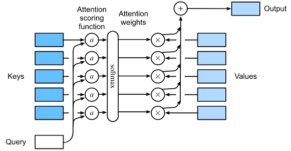
数学上, 假设我们有 query $q \in R^q$ 以及 $m$ key-value 对 $(k_1, v_1), …, (k_m, v_m)$, 对所有的 $k_i \in R^k$ 和 $v_i \in R^v$。 注意力池化 $f$ 实例化为 values 的加权和:
\[f(q, (k_1, v_1), ..., (k_m, v_m)) = \sum_{i=1}^m \alpha(q, k_i)v_i \in R^v \tag{10.3.1}\]其中,query $q$ 和 key $k_i$ 的注意力权重(标量)是通过 注意力评分函数 $a$ 的softmax操作计算的,该函数将两个向量映射为一个标量:
\[\alpha(q, k_i) = softmax(a(q, k_i)) = \frac{\exp(a(q, k_i))}{\sum_{j=1}^m \exp(a(q, k_j))} \in R \tag{10.3.2}\]可以看出,不同的注意力评分函数选择导致不同的注意力池化行为。在本节中,我们将介绍两个流行的评分函数,稍后我们将使用它们来开发更复杂的注意力机制。
1
2
3
4
import math
import torch
from torch import nn
from d2l import torch as d2l
Masked Softmax Operation
正如我们刚才提到的,softmax操作用于输出 attention 权重的概率分布。在某些情况下,并不是所有的 values 都应该用于送入 注意力池化。 例如,为了在第9.5节中进行高效的 minibatch处理,一些文本序列被 使用不具有意义的特殊标记填充。为了获得 仅将有意义的 tokens 作为 values 的注意力池化,我们可以指定一个有效的序列长度(以 tokens 数量为单位),以便在计算softmax时过滤掉超出这个指定范围的那些值。通过这种方式,我们可以在下面的 masked_softmax 函数中实现这样的 masked softmax 操作,其中任何超过有效长度的值都被 masked 为零。
1
2
3
4
5
6
7
8
9
10
11
12
13
14
15
16
17
18
19
20
21
22
23
24
25
def masked_softmax(X, valid_lens):
    """
    args:
        X : (batch, rows, columns)
        valid_lens :  batch中各个样本要mask的长度
    return:
        mask 之后的X 的 softmax 结果
    """
    """Perform softmax operation by masking elements on the last axis."""
    # `X`: 3D tensor, `valid_lens`: 1D or 2D tensor
    if valid_lens is None:
        return nn.functional.softmax(X, dim=-1)
    else:
        shape = X.shape
        if valid_lens.dim() == 1:
            #--- 因为输入的valid_lens是batch对应的,现在要把它变成列对应的, 所以需要复制它 ---
            valid_lens = torch.repeat_interleave(valid_lens, shape[1])
        else:
            valid_lens = valid_lens.reshape(-1)
        # On the last axis, replace masked elements with a very large negative
        # value, whose exponentiation outputs 0
        #--- X.reshape(-1, shape[-1]) 这个操作其实是将batch变成了行的形式 ---
        X = d2l.sequence_mask(X.reshape(-1, shape[-1]), valid_lens, value=-1e6)
        #--- 再将mask后的结果还原成batch的形式 ---
        return nn.functional.softmax(X.reshape(shape), dim=-1)
为了演示这个函数是如何工作的,请考虑两个 $2 \times 4$ 矩阵样本的minibatch,其中这两个样本的有效长度分别是2和3。作为masked softmax操作的结果,超过有效长度的值都被 masked 为零。
1
masked_softmax(torch.rand(2, 2, 4), torch.tensor([2, 3]))
输出:
1
2
3
4
5
array([[[0.488994  , 0.511006  , 0.        , 0.        ],
        [0.4365484 , 0.56345165, 0.        , 0.        ]],

       [[0.288171  , 0.3519408 , 0.3598882 , 0.        ],
        [0.29034296, 0.25239873, 0.45725837, 0.        ]]])
类似地,我们也可以使用一个二维张量来指定每个矩阵示例中每一行的有效长度。
1
masked_softmax(torch.rand(2, 2, 4), torch.tensor([[1, 3], [2, 4]]))
输出:
1
2
3
4
5
tensor([[[1.0000, 0.0000, 0.0000, 0.0000],
         [0.3174, 0.3988, 0.2837, 0.0000]],

        [[0.4621, 0.5379, 0.0000, 0.0000],
         [0.2578, 0.2652, 0.2603, 0.2167]]])
Additive Attention
一般来说,当queries和键keys是不同长度的向量时,我们可以使用加性注意力作为评分函数。给定一个 query $q \in \mathbb{R}^q$ 以及 一个 key $k \in \mathbb{R}^k$, 加性注意力评分函数如下:
\[a(q, k) = w_v^T \tanh(W_q q + W_k k) \in \mathbb{R} \tag{10.3.3}\]其中可学习参数 $W_q \in \mathbb{R}^{h \times q}$, $W_k \in \mathbb{R}^{h \times k}$, 以及 $w_v \in \mathbb{R}^h$。等价于 (10.3.3), query 和 key 被 concatenated 并输入到具有单个隐藏层的MLP中,该隐藏层的隐藏单元数为 $h$ ,这是一个超参数。通过使用 tanh 作为激活函数 并且 不使用 bias 项,我们在下面实现加性注意力。
1
2
3
4
5
6
7
8
9
10
11
12
13
14
15
16
17
18
19
20
21
22
23
24
25
26
27
28
29
30
31
32
33
34
35
36
37
38
39
40
41
class AdditiveAttention(nn.Module):
    def __init__(self, key_size, query_size, num_hiddens, dropout, **kwargs):
        super(AdditiveAttention, self).__init__(**kwargs)
        self.W_k = nn.Linear(key_size, num_hiddens, bias=False)
        self.W_q = nn.Linear(query_size, num_hiddens, bias=False)
        self.w_v = nn.Linear(num_hiddens, 1, bias=False)
        self.dropout = nn.Dropout(dropout)

    def forward(self, queries, keys, values, valid_lens):
        """
        args:
            queries : shape(batch_size, no. of queries, queries_features)
            keys: shape(batch_size, no. of key-value pairs, keys_features)
            values: shape(batch_size, no. of key-value pairs, values_features)
        return:
            outputs.shape : (batch_size, no. of queries, values_ features)
        """
        # queries.shape: (2, 1, 10) -> (2, 1, 8)
        # keys.shape: (2, 10, 2) -> (2, 10, 8)
        queries, keys = self.W_q(queries), self.W_k(keys)

        # After dimension expansion, shape of `queries`: (`batch_size`, no. of
        # queries, 1, `num_hiddens`) and shape of `keys`: (`batch_size`, 1,
        # no. of key-value pairs, `num_hiddens`). Sum them up with broadcasting
        # 通过广播机制将线性变换后的queries和keys相加
        # queries.shape: (2, 1, 8) -> (2, 1, 1, 8)
        # keys.shape: (2, 10, 2) -> (2, 1, 10, 8)
        features = queries.unsqueeze(2) + keys.unsqueeze(1)
        features = torch.tanh(features)
        # There is only one output of `self.w_v`, so we remove the last
        # one-dimensional entry from the shape. Shape of `scores`:
        # (`batch_size`, no. of queries, no. of key-value pairs)
        # scores.shape: (2, 1, 10)
        scores = self.w_v(features).squeeze(-1)
        # self.attention_weights.shape: (2, 1, 10)
        self.attention_weights = masked_softmax(scores, valid_lens)
        # Shape of `values`: (`batch_size`, no. of key-value pairs, value
        # dimension)
        # output.shape: (2, 1, 4)
        return torch.bmm(self.dropout(self.attention_weights), values)
让我们使用一个简单的样本演示一下上面的 AdditiveAttention 类, 其中 queries, keys, 和 values 的形状 (batch size, number of stepsor sequence length in tokens, feature size) 分别为 (2, 1, 20), (2, 10, 2) 和 (2, 10, 4)。attention pooling 输出的形状为 ((batch size, number of steps for queries, feature size for values))
1
2
3
4
5
6
7
8
queries, keys = torch.normal(0, 1, (2, 1, 20)), torch.ones((2, 10, 2))
# The two value matrices in the `values` minibatch are identical
values = torch.arange(40, dtype=torch.float32).reshape(1, 10, 4).repeat(2, 1, 1)
valid_lens = torch.tensor([2, 6])

attention = AdditiveAttention(key_size=2, query_size=20, num_hiddens=8, dropout=0.1)
attention.eval()
attention(queries, keys, values, valid_lens)
输出:
1
2
3
tensor([[[ 2.0000,  3.0000,  4.0000,  5.0000]],

        [[10.0000, 11.0000, 12.0000, 13.0000]]], grad_fn=<BmmBackward0>)
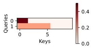
尽管加性注意力包含了可学习的参数,但由于本例中的每个 key 都是相同的,因此注意力权重是均匀的,由valid_lens决定。
1
d2l.show_heatmaps(attention.attention_weights.reshape((1, 1, 2, 10)), xlabel='Keys', ylabel='Queries')
Scaled Dot-Product Attention
一个计算效率更高的 scoring function 设计可以是简单的点积。然而,点积运算要求 query 和 key 具有相同的向量长度,比如 $d$。假设 query 和 key 的所有元素 都是独立的随机变量,其均值和单位方差均为零。两个向量的点积的均值为零,方差为 $d$。scaled dot-product 评分函数:
\[a(q, k) = q^T k / \sqrt{d} \tag{10.3.4}\]点积再除以 $\sqrt{d}$。 在实际操作中,为了提高效率,我们通常会考虑使用 minibatch,例如计算 $n$ queries 和 $m$ key-value pairs的注意力,其中 queries 和 keys 的长度为 $d$,values 的长度为 $v$。queries $Q \in \mathbb{R}^{n \times d}$, keys $K \in \mathbb{R}^{m \times d}$ 和 values $V \in \mathbb{R}^{m \times v}$ 的 scaled dot-product attention 为:
\[softmax (\frac{QK^T}{\sqrt{d}})V \in \mathbb{R}^{n \times v} \tag{10.3.5}\]在下面的 scaled dot product attention 的实现中, 我们使用 dropout 进行模型正则化。
1
2
3
4
5
6
7
8
9
10
11
12
13
14
15
16
17
18
#@save
class DotProductAttention(nn.Module):
    """Scaled dot product attention."""
    def __init__(self, dropout, **kwargs):
        super(DotProductAttention, self).__init__(**kwargs)
        self.dropout = nn.Dropout(dropout)

    # Shape of `queries`: (`batch_size`, no. of queries, `d`)
    # Shape of `keys`: (`batch_size`, no. of key-value pairs, `d`)
    # Shape of `values`: (`batch_size`, no. of key-value pairs, value
    # dimension)
    # Shape of `valid_lens`: (`batch_size`,) or (`batch_size`, no. of queries)
    def forward(self, queries, keys, values, valid_lens=None):
        d = queries.shape[-1]
        # Set `transpose_b=True` to swap the last two dimensions of `keys`
        scores = torch.bmm(queries, keys.transpose(1, 2)) / math.sqrt(d)
        self.attention_weights = masked_softmax(scores, valid_lens)
        return torch.bmm(self.dropout(self.attention_weights), values)
为了演示上面的DotProductAttention类,我们使用与前面加性注意力的简单示例相同的key、value和valid lengths。
1
2
3
4
queries = torch.normal(0, 1, (2, 1, 2))
attention = DotProductAttention(dropout=0.5)
attention.eval()
attention(queries, keys, values, valid_lens)
输出:
1
2
3
tensor([[[ 2.0000,  3.0000,  4.0000,  5.0000]],

        [[10.0000, 11.0000, 12.0000, 13.0000]]])
与加性注意力示例一样,由于 key 中包含的元素相同,不能通过 query 加以区分,因此获得了均匀的的注意力权重。
1
2
d2l.show_heatmaps(attention.attention_weights.reshape((1, 1, 2, 10)),
                  xlabel='Keys', ylabel='Queries')

Summary
- 我们可以用 values 的加权平均值来计算注意力池化的输出,不同的注意力评分函数的选择导致不同的注意力池化行为。
- 当 queries 和 keys 是不同长度的向量时,我们可以使用加法注意评分函数。当两者长度相同时,scaled dot-product 注意力评分函数的计算效率更高。
Exercises
- 修改简单示例中的 key 并可视化注意权重。加性注意力和 scaled dot-product 注意力是否仍然输出相同的注意力权重?为什么?
- 仅使用矩阵乘法,你能为具有不同向量长度的 queries 和 keys 设计一个新的评分函数吗?
- 当 queries 和 keys 具有相同的向量长度时,向量和是否比点积更好地设计得分函数?为什么?
-
Previous
【d2l】Attention Pooling: Nadaraya-Watson Kernel Regression -
Next
【深度学习】CLIP: Connecting Text and Images