Torch

torch.add

torch.add(input, alpha=1, other, out=None)

input (Tensor) – 第一个输入的向量
alpha (Number) - 系数
other (Tensor) – 第二个输入的向量

t = torch.tensor([2., 2.])
decay = 0.9
t1 = torch.tensor([3., 3.])
t.mul_(decay).add_(1-decay, t1)

输出：
tensor([2.1000, 2.1000])

当输入是一个数的时候，默认是other

当输入两个数的时候，默认第一个是alpha，第二个是tensor

torch.scatter

scatter_(dim, index, src) → Tensor

dim (int)-索引的轴向
index (LongTensor)-要散布的元素的索引，可以是空的或者和src的size相同。如果是空，这个操作会返回一个单位阵。
src (Tensor or float)-如果值没有被指定的话，要散布的源元素，。
将src中的所有值按照index确定的索引写入本tensor中。其中索引是根据给定的dimension，dim按照gather()描述的规则来确定。

注意，index的值必须是在0到(self.size(dim)-1)之间

>>> x = torch.rand(2, 5)
>>> x
tensor([[ 0.3992,  0.2908,  0.9044,  0.4850,  0.6004],
        [ 0.5735,  0.9006,  0.6797,  0.4152,  0.1732]])

1) dim = 0，分别对每列填充：

>>> torch.zeros(3, 5).scatter_(0, torch.tensor([[0, 1, 2, 0, 0], [2, 0, 0, 1, 2]]), x)
tensor([[ 0.3992,  0.9006,  0.6797,  0.4850,  0.6004],
        [ 0.0000,  0.2908,  0.0000,  0.4152,  0.0000],
        [ 0.5735,  0.0000,  0.9044,  0.0000,  0.1732]])

将index的矩阵称为tmp = [[0, 1, 2, 0, 0], [2, 0, 0, 1, 2]]；将最终的 3 * 5的矩阵，暂且称为result。

对于tmp[0][0] = 0 -> 取x中x[0][0] = 0.3992，将其插入到result第0列的第0个位置，result[0][0] = 0.3992；

对于tmp[0][1] = 1 -> 取x中x[0][1] = 0.2908，将其插入到result第1列的第1个位置，result[1][1] = 0.2908；

对于tmp[0][2] = 2 -> 取x中x[0][1] = 0.9044，将其插入到result第2列的第2个位置，result[2][2] = 0.9044；

……

对于tmp[1][0] = 2 -> 取x中x[1][0] = 0.5735，将其插入到result第0列的第2个位置，result[2][0] = 0.5735；

对于tmp[1][1] = 0 -> 取x中x[1][1] = 0.9006，将其插入到result第1列的第0个位置，result[0][1] = 0.9006。

2) dim = 1，分别对每行填充

>>> z = torch.zeros(2, 4).scatter_(1, torch.tensor([[2], [3]]), 1.23)
>>> z
tensor([[ 0.0000,  0.0000,  1.2300,  0.0000],
        [ 0.0000,  0.0000,  0.0000,  1.2300]])

tmp = [[2], [3]]

将result[0][2]和result[1][3]中的值填成1.23

torch.cat

torch.cat(inputs, dimension=0) → Tensor

inputs (sequence of Tensors) – 可以是任意相同Tensor 类型的python 序列
dimension (int, optional) – 沿着此维连接张量序列

Example:

l = []
for i in range(2):
    l.append(torch.randn((1, 3, 4, 4)))
print(torch.cat(l, 0).size())

输出：
torch.Size([2, 3, 4, 4])

如果一维且不指定维度，那么相当于拼接在后边。

torch.reshape

torch.reshape(input, shape) → Tensor

返回一个和输入有相同的数据和元素数量的tensor，但是是指定的形状。

如果可能的话，返回输入的视图。否则返回副本。

连续的输入以及兼容步长的输入可以不用以副本的方式返回，但是你不应该依赖于这个特性。

单个维度可能为-1，在这种情况下，它由剩余维度和输入中的元素数量推断而来。

PyTorch view和reshape的区别

相同之处

都可以用来重新调整 tensor 的形状。

不同之处

view 函数只能用于 contiguous 后的 tensor 上，也就是只能用于内存中连续存储的 tensor。如果对 tensor 调用过 transpose, permute 等操作的话会使该 tensor 在内存中变得不再连续，此时就不能再调用 view 函数。因此，需要先使用 contiguous 来返回一个 contiguous copy。
reshape 则不需要依赖目标 tensor 是否在内存中是连续的。

torch.max

torch.max(input) → Tensor

返回输入tensor中所有元素的最大值

torch.max(input, dim, keepdim=False, out=None) -> (Tensor, LongTensor)

返回一个元组(值，索引)，其中值是给定维度中输入张量的每一行的最大值。索引是找到每个最大值(argmax)的索引位置

torch.max(input, other, *, out=None) → Tensor

见 torch.maximum().

torch.maximum

torch.maximum(input, other, *, out=None) → Tensor

计算按元素计算 input 和 other 的最大值。

如果被比较的元素中有一个是NaN，则返回该元素。对于具有复数dtype的张量，不支持maximum()。

参数：

input (Tensor) – the input tensor.
other (Tensor) – the second input tensor
out (Tensor, optional) – the output tensor.

torch.argmax

torch.argmax(input) → LongTensor

返回输入张量中所有元素的最大值的索引。

这是torch.max()返回的第二个值。有关此方法的确切语义，请参阅其文档。

如果有多个最小值，则返回第一个最小值的索引。

参数：

input (Tensor) – the input tensor.

>>> a = torch.randn(4, 4)
>>> a
tensor([[ 1.3398,  0.2663, -0.2686,  0.2450],
        [-0.7401, -0.8805, -0.3402, -1.1936],
        [ 0.4907, -1.3948, -1.0691, -0.3132],
        [-1.6092,  0.5419, -0.2993,  0.3195]])
>>> torch.argmax(a)
tensor(0)

Example:

torch.argmax(input, dim, keepdim=False) → LongTensor

返回跨维度张量的最大值的索引。

这是torch.max()返回的第二个值。有关此方法的确切语义，请参阅其文档。

参数：

input (Tensor) – the input tensor.
dim (int) – the dimension to reduce. If None, the argmax of the flattened input is returned.
keepdim (bool) – whether the output tensor has dim retained or not. Ignored if dim=None.

Example:

>>> a = torch.randn(4, 4)
>>> a
tensor([[ 1.3398,  0.2663, -0.2686,  0.2450],
        [-0.7401, -0.8805, -0.3402, -1.1936],
        [ 0.4907, -1.3948, -1.0691, -0.3132],
        [-1.6092,  0.5419, -0.2993,  0.3195]])
>>> torch.argmax(a, dim=1)
tensor([ 0,  2,  0,  1])

torch.min

torch.min(input) → Tensor

返回输入张量中所有元素的最小值。

torch.min(input, dim, keepdim=False, *, out=None) -> (Tensor, LongTensor)

类似与torch.max

torch.min(input, other, *, out=None) → Tensor

See torch.minimum().

torch.minimum

torch.minimum(input, other, *, out=None) → Tensor

与 torch.maximum相似。

torch.sum

torch.sum(input, *, dtype=None) → Tensor

返回输入张量中所有元素的和。

参数：

input (Tensor) – 输入的张量

torch.sum(input, dim, keepdim=False, *, dtype=None) → Tensor

返回给定维度dim中输入张量的每一行的和。如果dim是维度列表，则对所有维度进行归约。

torch.squeeze

torch.squeeze(input, dim=None, out=None) → Tensor

删除size是1的维度

比如， input的shape是$(A \times 1 \times B \times C \times 1 \times D)$， output的shape是$A \times B \times C \times D$

>>> x = torch.zeros(2, 1, 2, 1, 2)
>>> x.size()
torch.Size([2, 1, 2, 1, 2])
>>> y = torch.squeeze(x)
>>> y.size()
torch.Size([2, 2, 2])
>>> y = torch.squeeze(x, 0)
>>> y.size()
torch.Size([2, 1, 2, 1, 2])
>>> y = torch.squeeze(x, 1)
>>> y.size()
torch.Size([2, 2, 1, 2])

torch.unsqueeze(input, dim, out=None) → Tensor

返回一个新tensor在特定位置插入一个维度

input (Tensor) – the input tensor.
dim (python:int) – 要插入那一维的索引
out (Tensor, optional) – the output tensor.

torch.chunk

torch.chunk(input, chunks, dim=0) → List of Tensors

将Tensor拆分为特定数量的块。

如果沿着给定维度dim的张量大小无法被块整除，则最后一个块将更小。

input (Tensor) – the tensor to split
chunks (python:int) – number of chunks to return
dim (python:int) – dimension along which to split the tensor

torch.arange

torch.arange(start, end, step=1, out=None) → Tensor

包含从start到end，以step为步长的一组序列值(默认步长为1)。

start (float) – 序列的起始点
end (float) – 序列的终止点
step (float) – 相邻点的间隔大小
out (Tensor, optional) – 结果张量

torch.clamp

torch.clamp(input, min, max, out=None) → Tensor

将input的所有元截断到放到范围[min, max]，返回结果tensor

\[y_i = \begin{cases} min & {if x_i < min} \\ x_i & {if min \leq x_i \leq max}\\ max & {if x_i \geq max} \end{cases}\]

torch.clip

torch.clip(input, min, max, *, out=None) → Tensor

torch.clamp() 的别名。

torch.var

torch.var(input, dim, keepdim=False, unbiased=True, out=None) → Tensor

返回输入tensor在给定维度dim的方差。

如果keepdim是True，输出的tensor尺寸和input一样除非维度dim尺寸为1。否则， dim会被压缩掉，导致输出tensor的维数减少1（或len（dim））。

如果unbiaded为False，则将通过有偏估计量计算方差。否则，将使用bessel更正。

例子：

>>> a = torch.randn(4, 4)
>>> a
tensor([[-0.3567,  1.7385, -1.3042,  0.7423],
        [ 1.3436, -0.1015, -0.9834, -0.8438],
        [ 0.6056,  0.1089, -0.3112, -1.4085],
        [-0.7700,  0.6074, -0.1469,  0.7777]])
>>> torch.var(a, 1)
tensor([ 1.7444,  1.1363,  0.7356,  0.5112])

torch.mean(input, dim, keepdim=False, out=None) → Tensor

和var相似，只不过计算的是均值。

torch.empty

torch.empty(*size, out=None, dtype=None, layout=torch.strided, device=None, requires_grad=False, pin_memory=False) → Tensor

返回一个没有被初始化数据的Tensor。

Tensor的形状为参数size。

size (python:int…)：一个整数序列定义输出Tensor的形状，可以是一个参数变量，也可以是一个list或者tuple集合。
out(Tensor, optional) ：输出的Tensor
dtype (torch.dtype, optional)：需要返回的Tensor的数据类型。默认，如果是None，使用全局默认（见torch.set_default_tensor_type()）
layout (torch.layout, optional)：需要返回Tensor的布局。默认：torch.strided。

当输入一些不带keywords的参数时，默认都是size的参数，其他参数使用默认参数。

torch.rand

torch.normal(mean, std, *, generator=None, out=None) → Tensor

返回一个采样自给定均值和方差的正态分布的Tensor

torch.rand(*size, out=None, dtype=None, layout=torch.strided, device=None, requires_grad=False) → Tensor

返回一个采样自正态分布的tensor，值[0, 1)

torch.randint(low=0, high, size, *, generator=None, out=None, dtype=None, layout=torch.strided, device=None, requires_grad=False) → Tensor

返回一个Tensor采样自low到high均匀分布的整数。

torch.randn(*size, out=None, dtype=None, layout=torch.strided, device=None, requires_grad=False) → Tensor

返回一个采样自标准正态分布的Tensor

产生噪声的方式

np.random.normal(0, 1, (imgs.shape[0], opt.latent_dim))

// 生成一个形状为(batch_size, nz, 1, 1)的Tensor
torch.randn(batch_size, nz, 1, 1, device=device)

numpy.random.normal(loc=0.0, scale=1.0, size=None)

参数的意义为：

　　loc:float

　　概率分布的均值，对应着整个分布的中心center

　　scale:float

　　概率分布的标准差，对应于分布的宽度，scale越大越矮胖，scale越小，越瘦高

　　size:int or tuple of ints

　　输出的shape，默认为None，只输出一个值

　　我们更经常会用到np.random.randn(size)所谓标准正态分布（μ=0, σ=1），对应于np.random.normal(loc=0, scale=1, size)

torch.rand(*sizes, out=None) → Tensor

返回一个张量，包含了从区间[0, 1)的均匀分布中抽取的一组随机数。张量的形状由参数sizes定义。

参数:

sizes (int…) - 整数序列，定义了输出张量的形状
out (Tensor, optinal) - 结果张量

torch.randn(*sizes, out=None) → Tensor

返回一个张量，包含了从标准正态分布（均值为0，方差为1，即高斯白噪声）中抽取的一组随机数。张量的形状由参数sizes定义。

参数:

sizes (int…) - 整数序列，定义了输出张量的形状
out (Tensor, optinal) - 结果张量

Note：在生成噪声后，要将噪声送入cuda

torch.norm

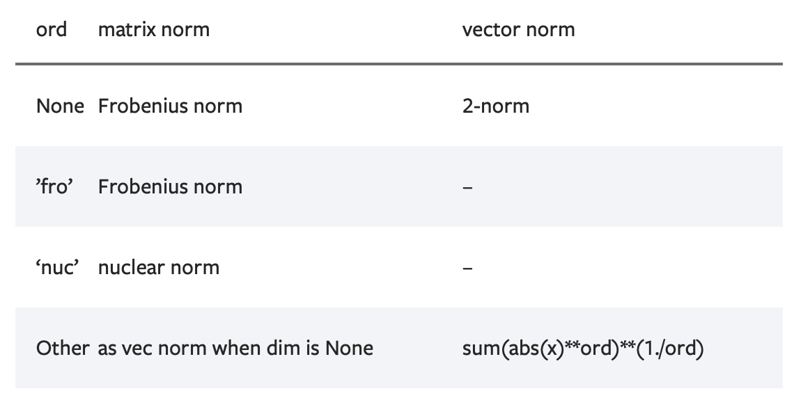
torch.norm(input, p=’fro’, dim=None, keepdim=False, out=None, dtype=None)

返回一个给定Tensor的矩阵范数或者向量范数

input (Tensor) – the input tensor
p (python:int, python:float, inf, -inf, ‘fro’, ‘nuc’, optional) – 范数计算中的幂指数值。默认为’fro’

dim (int，2-tuple，2-list， optional): 指定计算的维度。如果是一个整数值，向量范数将被计算；如果是一个大小为2的元组，矩阵范数将被计算；如果为None，当输入tensor只有两维时矩阵计算矩阵范数；当输入只有一维时则计算向量范数。如果输入tensor超过2维，向量范数将被应用在最后一维
keepdim（bool，optional）：指明输出tensor的维度dim是否保留。如果dim=None或out=None,则忽略该参数。默认值为False，不保留。

>>> import torch
>>> a = torch.arange(9, dtype=torch.float) - 4
>>> a
tensor([-4., -3., -2., -1.,  0.,  1.,  2.,  3.,  4.])
>>> b = a.reshape(3,3)
>>> b
tensor([[-4., -3., -2.],
        [-1.,  0.,  1.],
        [ 2.,  3.,  4.]])
>>> torch.norm(a)
tensor(7.7460)
>>> torch.norm(b)
tensor(7.7460)

>>> torch.norm(a, float('inf'))
tensor(4.)
>>> torch.norm(b, float('inf'))
tensor(4.)

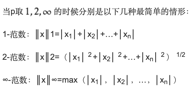
1）如果不指明p，则是计算Frobenius范数

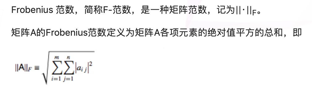
以上面的例子中a,b的结果都相同$7.7460 = \sqrt{（16*2 + 9*2 +4*2 + 1*2）}$

2）p = ‘inf’,则是求出矩阵或向量中各项元素绝对值中的最大值，所以为4

>>> c = torch.tensor([[1,2,3],[-1,1,4]], dtype=torch.float)
>>> c
tensor([[ 1.,  2.,  3.],
        [-1.,  1.,  4.]])
>>> torch.norm(c, dim=0)
tensor([1.4142, 2.2361, 5.0000])
>>> torch.norm(c, dim=0).size()
torch.Size([3])
>>> torch.norm(c, dim=1)
tensor([3.7417, 4.2426])
>>> torch.norm(c, p=1, dim=1)
tensor([6., 6.])

1）指定dim = 0，因为c的size() = (2,3),所以会去掉其dim=0，得到size()=(3)的结果，所以是纵向求值，计算Frobenius范数

2）p=1, dim=1 ：即是表示去掉维度1，使用1-范数，得到size()=(2)的结果。所以横向计算各个元素绝对值的和，为（[6,6]）

torch.mul 和 torch.matmul

torch.mul(input, other, out=None)

对应元素相乘，带有广播机制

>>> a = torch.randn(4, 1)
>>> a
tensor([[ 1.1207],
        [-0.3137],
        [ 0.0700],
        [ 0.8378]])
>>> b = torch.randn(1, 4)
>>> b
tensor([[ 0.5146,  0.1216, -0.5244,  2.2382]])
>>> torch.mul(a, b)
tensor([[ 0.5767,  0.1363, -0.5877,  2.5083],
        [-0.1614, -0.0382,  0.1645, -0.7021],
        [ 0.0360,  0.0085, -0.0367,  0.1567],
        [ 0.4312,  0.1019, -0.4394,  1.8753]])

torch.matmul(input, other, out=None) → Tensor

矩阵乘法，带有广播机制

当input是$(j \times 1 \times n \times m)$的tensor， other是一个$(k \times m \times p)$， out会是一个$(j \times k \times n \times p)$的tensor

torch.bmm

torch.bmm(input, mat2, out=None) → Tensor

对input和mat2中存储的矩阵执行批处理矩阵-矩阵乘积

input和mat2必须是三维的tensor，每个矩阵包含着相同数量的数据

如果input是一个$(b \times n \times m)$的tensor， mat2是一个$b \times m \times p$的tensor， out将是一个$(b \times n \times p)$的tensor。

torch.bmm和torch.matmul的区别

bmm只能进行矩阵乘法,也就是输入的两个tensor维度只能是(b×n×p), 第一维b代表batch_size
matmul可以进行张量乘法, 输入可以是高维.

torch.mv

torch.mv(input, vec, out=None) → Tensor

对input矩阵和vec向量执行矩阵-向量的乘法

如果input是一个$(n \times m)$的tensor， vec是一个尺寸为m的1维tensor，输出将会是一个尺寸为n的一维tensor

Note：这个函数没有广播机制

torch.eq

torch.eq(input, other, out=None) → Tensor

对比每个元素是否相等

第二个参数可以是一个数字或者是一个可以广播成第一个参数形状的张量。

返回一个torch.BoolTensor，如果相等，相应位置为True。

torch.dot

torch.dot(input, tensor) → Tensor

计算两个向量的内积

Example：

>>> torch.dot(torch.tensor([2, 3]), torch.tensor([2, 1]))
tensor(7)

torch.flip

torch.flip(input, dims) → Tensor

Example:

>>> x = torch.arange(8).view(2, 2, 2)
>>> x
tensor([[[ 0,  1],
         [ 2,  3]],

        [[ 4,  5],
         [ 6,  7]]])
>>> torch.flip(x, [0, 1])
tensor([[[ 6,  7],
         [ 4,  5]],

        [[ 2,  3],
         [ 0,  1]]])

torch.t

torch.t(input) → Tensor

期待的输入是一个小于等于2维的tensor，并且转置维度0和维度1

按原样返回0-D和1-D张量，并且2-D张量可以视为transpose（input，0，1）的简写函数

Example：

>>> x = torch.randn(())
>>> x
tensor(0.1995)
>>> torch.t(x)
tensor(0.1995)
>>> x = torch.randn(3)
>>> x
tensor([ 2.4320, -0.4608,  0.7702])
>>> torch.t(x)
tensor([.2.4320,.-0.4608,..0.7702])
>>> x = torch.randn(2, 3)
>>> x
tensor([[ 0.4875,  0.9158, -0.5872],
        [ 0.3938, -0.6929,  0.6932]])
>>> torch.t(x)
tensor([[ 0.4875,  0.3938],
        [ 0.9158, -0.6929],
        [-0.5872,  0.6932]])

torch.numel

torch.numel(input) → int

numer elements

返回输入tensor元素总数

Example：

>>> a = torch.randn(1, 2, 3, 4, 5)
>>> torch.numel(a)
120
>>> a = torch.zeros(4,4)
>>> torch.numel(a)
16

torch.full

torch.full(size, fill_value, *, out=None, dtype=None, layout=torch.strided, device=None, requires_grad=False) → Tensor

创建一个用 fill_value 填充的size张量。张量的 dtype 是由 fill_value 推导出来的。

参数：

size (int…) – 列表、元组或定义输出张量的形状（torch.Size）。
fill_value (Scalar) – 用来填充输出张量的值。
out (Tensor, optional) – 输出张量。
dtype (torch.dtype, optional) – 返回张量所需的数据类型。Default:如果为None，则使用全局默认值(see torch.set_default_tensor_type())。
layout (torch.layout, optional) – 返回张量所需的layout。Default: torch.strided。
device (torch.device, optional) – 返回张量的所需 device。
requires_grad (bool, optional) – 如果autograd应该记录对返回张量的操作。

torch.nonzero

torch.nonzero(input, *, out=None, as_tuple=False) → LongTensor or tuple of LongTensors

当 as_tuple 为 “False”(default)：

返回一个二维张量，其中每行是一个非零值的索引。

返回一个张量，其中包含 input 的所有非零元素的索引。结果中的每一行都包含 input 中一个非零元素的索引。结果按字典顺序排序，最后一个索引的变化最快(C风格)。

如果 input 的维数是 $n$，那么得到的索引张量 out 的大小是 $(z \times n)$，其中 $z$ 是 input 张量中非零元素的总数。

当 as_tuple 为 “True”：

返回一个由一维张量组成的元组，每个张量对应 input 的每个维度，每个张量包含 input 的所有非零元素的索引(在该维度中)。

如果 input 有 $n$ 维数，那么得到的元组包含 $n$ 个大小为 $z$ 的张量，其中 $z$ 是 input 张量中非零元素的总数。

作为一种特殊情况，当 input 为零维且标量值为非零时，它被视为一个只有一个元素的一维张量。

例子：

>>> torch.nonzero(torch.tensor([1, 1, 1, 0, 1]))
tensor([[ 0],
        [ 1],
        [ 2],
        [ 4]])
>>> torch.nonzero(torch.tensor([[0.6, 0.0, 0.0, 0.0],
                                [0.0, 0.4, 0.0, 0.0],
                                [0.0, 0.0, 1.2, 0.0],
                                [0.0, 0.0, 0.0,-0.4]]))
tensor([[ 0,  0],
        [ 1,  1],
        [ 2,  2],
        [ 3,  3]])
>>> torch.nonzero(torch.tensor([1, 1, 1, 0, 1]), as_tuple=True)
(tensor([0, 1, 2, 4]),)
>>> torch.nonzero(torch.tensor([[0.6, 0.0, 0.0, 0.0],
                                [0.0, 0.4, 0.0, 0.0],
                                [0.0, 0.0, 1.2, 0.0],
                                [0.0, 0.0, 0.0,-0.4]]), as_tuple=True)
(tensor([0, 1, 2, 3]), tensor([0, 1, 2, 3]))
>>> torch.nonzero(torch.tensor(5), as_tuple=True)
(tensor([0]),)

torch.save与torch.load

仅保存和加载模型参数

torch.save(the_model.state_dict(), PATH)

the_model = TheModelClass(*args, **kwargs)
the_model.load_state_dict(torch.load(PATH))

保存和加载整个模型

torch.save(the_model, PATH)
the_model = torch.load(PATH)

保存

def save_model(epoch, encoder, decoder, D):
    state = {'encoder': encoder.cpu().state_dict(),
             'decoder': decoder.cpu().state_dict(),
             'D':D.cpu().state_dict(),
             'epoch': epoch,}
    
    torch.save(state, 'VAE_GAN%d.pth' % epoch)

加载

try:
	state = torch.load('../input/resnet50/resnet50')
	net.load_state_dict(state['net'])
	best_accuracy = state['best_accuracy']
	best_val_accuracy = state['best_val_accuracy']
	losses = state['loss']
	accuracies = state['accuracy']
except:

	print("No checkpoint...")

torch.cuda()

.cuda()函数返回一个存储在CUDA内存中的复制，其中device可以指定cuda设备。但如果此storage对象早已在CUDA内存中存储，并且其所在的设备编号与cuda()函数传入的device参数一致，则不会发生复制操作，返回原对象。

参数

device (int) – 指定的GPU设备id. 默认为当前设备，即 torch.cuda.current_device()的返回值。
non_blocking (bool) – 如果此参数被设置为True, 并且此对象的资源存储在固定内存上(pinned memory)，那么此cuda()函数产生的复制将与host端的原storage对象保持同步。否则此参数不起作用。

torch.repeat_interleave

torch.repeat_interleave(input, repeats, dim=None) → Tensor

重复一个tensor的元素。

它和torch.Tensor.repeat()不同，但是和numpy.repeat相似。

input (Tensor) – 输入的tensor。
repeats (Tensor or int) – 每个元素重复的数量。 repeat广播以适应给定轴的形状。
dim (int, optional) – 重复元素的轴。默认 flatten 输入的array，返回一个平的array。

例子：

>>> x.repeat_interleave(2)
tensor([1, 1, 2, 2, 3, 3])
>>> y = torch.tensor([[1, 2], [3, 4]])
>>> torch.repeat_interleave(y, 2)
tensor([1, 1, 2, 2, 3, 3, 4, 4])
>>> torch.repeat_interleave(y, 3, dim=1)
tensor([[1, 1, 1, 2, 2, 2],
        [3, 3, 3, 4, 4, 4]])
>>> torch.repeat_interleave(y, torch.tensor([1, 2]), dim=0)
tensor([[1, 2],
        [3, 4],
        [3, 4]])

torch.argsort

torch.argsort(input, dim=-1, descending=False) → LongTensor

返回按值升序对给定维度张量排序的索引。

这是torch.sort()返回的第二个值。有关此方法的确切语义，请参阅其文档。

参数：

input (Tensor) – the input tensor.
dim (int, optional) – the dimension to sort along
descending (bool, optional) – controls the sorting order (ascending or descending)

Example：

>>> a = torch.randn(4, 4)
>>> a
tensor([[ 0.0785,  1.5267, -0.8521,  0.4065],
        [ 0.1598,  0.0788, -0.0745, -1.2700],
        [ 1.2208,  1.0722, -0.7064,  1.2564],
        [ 0.0669, -0.2318, -0.8229, -0.9280]])


>>> torch.argsort(a, dim=1)
tensor([[2, 0, 3, 1],
        [3, 2, 1, 0],
        [2, 1, 0, 3],
        [3, 2, 1, 0]])

torch.topk

torch.topk(input, k, dim=None, largest=True, sorted=True, *, out=None) -> (Tensor, LongTensor)

沿着给定维度返回input 张量的 k 个最大的元素

input(Tensor) - 输入的张量
k(int) - “top-k” 中的 k
dim(int, optional) - 沿着排序的维度
largest(bool, optional) - 选择返回最大的还是最小的元素
sorted(bool, optional) - 控制是否返回排序过后的元素

torch.where

torch.where(condition, x, y) → Tensor

返回一个tensor，其值从 x 或 y 中选择，依赖于 condition

\[out_i = \begin{cases} x_i & \text{if condition$_1$} \\ y_i & \text{otherwise} \end{cases}\]

借助 torch.where 找到矩阵中指定的数

torch.nonzero(torch.where(list_torch == element, torch.tensor(element), torch.tensor(0)))

原理就是借助nonzero函数，找到所有非0元素，首先是需要将不需要的元素变为0。

Tensor

resize

resize_(*sizes) → Tensor

让本tensor重新变为指定大小。如果元素数量比现在大，深层存储被重新改变大小以适应新的元素数量。如果元素数量更小，深层存储不变。现存的元素被保留，但是新的存储不会初始化。

警告这是一种低阶的方式。大多数情况你应该使用view()或者reshape()

尽量不要使用resize，会出现奇怪的问题，比如：

resize之前的tensor显示是这样：

而resize之后变成了噪声：

我猜测应该是维度混乱造成的。

expand

expand(*sizes) → Tensor

返回一个新的Tensor，将Tensor单个维度扩大为更大的尺寸。

给一个维度传入-1表示不改变这个维度的size

Tensor可以被扩展为一个更大维度，并且新的维度会添加在最前。

扩大tensor不需要分配新内存，只是仅仅新建一个tensor的视图，其中通过将stride设为0，一维将会扩展位更高维。任何一个一维的在不分配新内存情况下可扩展为任意的数值。

x = torch.Tensor([[1], [2], [3]])
print "x.size():",x.size()

y=x.expand( 3,4 )

print "x.size():",x.size()
print "y.size():",y.size()

print x
print y

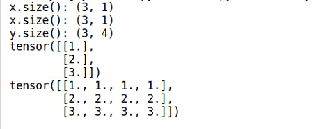
Note：使用expand()函数的时候，x自身不会改变，因此需要将结果重新赋值。

expand_as

expand_as(other) → Tensor

将这个tensor扩展成和other大小一样的tensor。

slef.expand_as(other)等价于self.expand(other.size())

repeat

repeat(*sizes) → Tensor

按照给定维度重复这个Tensor。

不像expand()，这个函数复制Tensor的数据。

类似于numpy.tile。

Examples:

x = torch.tensor([1, 2, 3])
print(x.repeat(4, 2,1).size())
x.repeat(4, 2, 1)


torch.Size([4, 2, 3])
tensor([[[1, 2, 3],
         [1, 2, 3]],

        [[1, 2, 3],
         [1, 2, 3]],

        [[1, 2, 3],
         [1, 2, 3]],

        [[1, 2, 3],
         [1, 2, 3]]])

就是沿着这个轴复制。比如说 repeat(4, 2) 就是沿着x轴复制四次，沿着y轴复制两次。

permute

permute(*dims) → Tensor

改变这个Tensor维度的序列

*dims (python:int…) – 想要的维度顺序

Example:

>>> x = torch.randn(2, 3, 5)
>>> x.size()
torch.Size([2, 3, 5])
>>> x.permute(2, 0, 1).size()
torch.Size([5, 2, 3])

new

torch.tensor.new(*size)

创建一个新的size大小的tensor

Example：

a = torch.randn(2, 3)
print(a)
b = a.new(a.size()[0])
print(b)
c = a.new(a.size()[1])
print(c)

输出：
tensor([[-1.2315, -0.7650, 0.9456],
[ 0.5871, -0.4789, -0.0105]])
tensor([0., 0.])
tensor([ 0.0000e+00, 0.0000e+00, -3.1534e-21])

masked_fill

Tensor.masked_fill_(mask, value)

当 mask 为 True 的时候，使用 value 填充 self Tensor的元素。 mask 必须可广播成潜在向量的形状。

mask (BoolTensor)：布尔mask
value (float) – 要填充的 value

torch.distributions

torch.distributions.beta.Beta

torch.distributions.beta.Beta(concentration1, concentration0, validate_args=None)

有concentration1和concentration0参数化的Beta分布

>>> m = Beta(torch.tensor([0.5]), torch.tensor([0.5]))
>>> m.sample()  # Beta distributed with concentration concentration1 and concentration0
tensor([ 0.1046])

torch.backends.cudnn

cuDNN使用非确定性算法，并且可以使用torch.backends.cudnn.enabled = False来进行禁用.

如果设置为torch.backends.cudnn.enabled =True，说明设置为使用使用非确定性算法.

然后再设置：

torch.backends.cudnn.benchmark = true

那么cuDNN使用的非确定性算法就会自动寻找最适合当前配置的高效算法，来达到优化运行效率的问题

一般来讲，应该遵循以下准则：

如果网络的输入数据维度或类型上变化不大，设置 torch.backends.cudnn.benchmark = true 可以增加运行效率；
如果网络的输入数据在每次 iteration 都变化的话，会导致 cnDNN 每次都会去寻找一遍最优配置，这样反而会降低运行效率。

所以我们经常看见在代码开始出两者同时设置：

torch.backends.cudnn.enabled = True torch.backends.cudnn.benchmark = True

torch.flatten

torch.flatten(input, start_dim=0, end_dim=-1) → Tensor

input(Tensor) – 输入的张量
start_dim (int) – flatten开始的维度
end_dim (int) – flatten的结束的维度

torch.meshgrid

类似numpy中meshgrid。

二维坐标系中,X轴可以取三个值1,2,3, Y轴可以取三个值7,8, 请问可以获得多少个点的坐标?

显而易见是6个:

(1,7)(2,7)(3,7) (1,8)(2,8)(3,8)

np.meshgrid()就是干这个的!

#coding:utf-8
import numpy as np
# 坐标向量
a = np.array([1,2,3])
# 坐标向量
b = np.array([7,8])
# 从坐标向量中返回坐标矩阵
# 返回list,有两个元素,第一个元素是X轴的取值,第二个元素是Y轴的取值
res = np.meshgrid(a,b)
#返回结果: [array([ [1,2,3] [1,2,3] ]), array([ [7,7,7] [8,8,8] ])]

同理还可以生成更高维度的坐标矩阵

torch.einsum

energy  = torch.einsum("nqhd, hkhd->nhqk", [queries, keys])

queries shape: (N, query_len, heads, head_dim)
key shape: (N, key_len, heads, head_dim)
energy shape: (N, haeds, query_len, key_len)

它就等价于

queries = queries.reshape(N * heads, quiery_len, head_dim)
keys = keys.reshape(N * heads, key_len, head_dim)
energy = torch.bmm(queries, keys.permute(0, 2, 1))

torch.tril

torch.tril(input, diagonal=0, *, out=None) → Tensor

参数：

input (Tensor) – 输入张量.
diagonal (int, optional)

返回input 矩阵的下三角部分，返回张量 out 的其它部分设为 0。

矩阵的下三角形部分定义为对角线和对角线以下的元素。

参数diagonal 如果等于0，所有对角线和对角线以下的元素保留。如果 diagonal 大于0，则有更多的对角线以上的元素被保留；如果 diagonal 小于0，将会有更少的对角线以下的元素被保留。如下面例子所示：

>>> a = torch.randn(3, 3)
>>> a
tensor([[-1.0813, -0.8619,  0.7105],
        [ 0.0935,  0.1380,  2.2112],
        [-0.3409, -0.9828,  0.0289]])
>>> torch.tril(a)
tensor([[-1.0813,  0.0000,  0.0000],
        [ 0.0935,  0.1380,  0.0000],
        [-0.3409, -0.9828,  0.0289]])

>>> b = torch.randn(4, 6)
>>> b
tensor([[ 1.2219,  0.5653, -0.2521, -0.2345,  1.2544,  0.3461],
        [ 0.4785, -0.4477,  0.6049,  0.6368,  0.8775,  0.7145],
        [ 1.1502,  3.2716, -1.1243, -0.5413,  0.3615,  0.6864],
        [-0.0614, -0.7344, -1.3164, -0.7648, -1.4024,  0.0978]])
>>> torch.tril(b, diagonal=1)
tensor([[ 1.2219,  0.5653,  0.0000,  0.0000,  0.0000,  0.0000],
        [ 0.4785, -0.4477,  0.6049,  0.0000,  0.0000,  0.0000],
        [ 1.1502,  3.2716, -1.1243, -0.5413,  0.0000,  0.0000],
        [-0.0614, -0.7344, -1.3164, -0.7648, -1.4024,  0.0000]])
>>> torch.tril(b, diagonal=-1)
tensor([[ 0.0000,  0.0000,  0.0000,  0.0000,  0.0000,  0.0000],
        [ 0.4785,  0.0000,  0.0000,  0.0000,  0.0000,  0.0000],
        [ 1.1502,  3.2716,  0.0000,  0.0000,  0.0000,  0.0000],
        [-0.0614, -0.7344, -1.3164,  0.0000,  0.0000,  0.0000]])

torch.addmm

torch.addmm(input, mat1, mat2, *, beta=1, alpha=1, out=None) → Tensor

实现矩阵 mat1 和 mat2 的矩阵乘法。矩阵 input 再被加到最后的结果上。

如果 mat1 是一个 ($n \times m$) 的张量， mat2 是一个 ($m \times p$) 的张量， input 必须是一个可广播成 ($n \times p$) 的张量。

\[out = \beta input + \alpha(mat1_i @ mat2_i)\]

torch.gather

沿dim指定的轴收集值。

对于一个三维张量，输出是为：

out[i][j][k] = input[index[i][j][k]][j][k]  # if dim == 0
out[i][j][k] = input[i][index[i][j][k]][k]  # if dim == 1
out[i][j][k] = input[i][j][index[i][j][k]]  # if dim == 2

input 和 index 必须有相同的维数。对于所有 d != dim.out 的维度需要 index.size(d) <= input.size(d)。注意，input 和 index 不会相互广播。

在指定的轴上，根据 index 指定的下标，选择元素重组成一个新的 tensor，最后输出的 out 与index 的 size 是一样的。

torch.multinomial

torch.multinomial(input, num_samples, replacement=False, *, generator=None, out=None) → LongTensor

返回一个张量，输入 input 张量以 multinomial 概率分布采样 num_samples 个元素，返回其索引。

torch.randperm

torch.randperm(n, *, generator=None, out=None, dtype=torch.int64, layout=torch.strided, device=None, requires_grad=False, pin_memory=False) → Tensor

例子：

>>> torch.randperm(4)
tensor([2, 1, 0, 3])

Pytorch查看版本信息及NVDIA查看版本信息

torch._version_

查看pytorch版本信息

torch.version.cuda

查看cuda版本信息

nvcc –version

查看nvcc版本

Torch.nn

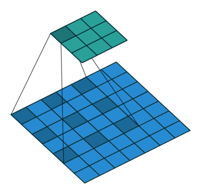
torch.nn.Conv2d

class torch.nn.Conv2d(in_channels, out_channels, kernel_size, stride=1, padding=0, dilation=1, groups=1, bias=True)

二维卷积层, 输入的尺度是(N, C_in,H,W)，输出尺度（N,C_out,H_out,W_out）的计算方式：

先定义几个参数

输入图片大小 W×W Filter大小 F×F 步长 S padding的像素数 P

\[N = \frac{(W − F + 2P )}{S}+1\]

输出图片大小为 N×N

bias(bool, optional): 如果是True，输出会学习一个bias。默认为True。
dilation：空洞卷积，控制卷积核两个点之间的空间

torch.nn.Softmax

torch.nn.Softmax(dim=None)

对一个n维的输入tensor使用Softmax，重新缩放它们，使得n维输出tensor的元素值在[0,1]并且和为1.

Softmax定义为：

\[Softmax(x_i) = \frac{exp(x_i)}{\sum_j exp(x_j)}\]

形状：

Input: (*) 其中*意味着，任意数量的额外维度
Output: (*) , 和输入相同的形状

一个和输入相同形状相同维度的tensor，值在[0, 1]

参数：

dim (python:int) – Softmax将要计算的那一维（沿着那一维的所有切片和为1）

例子：

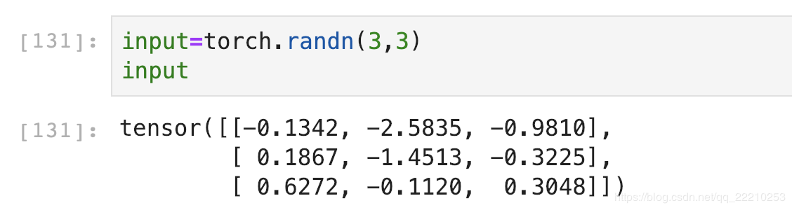
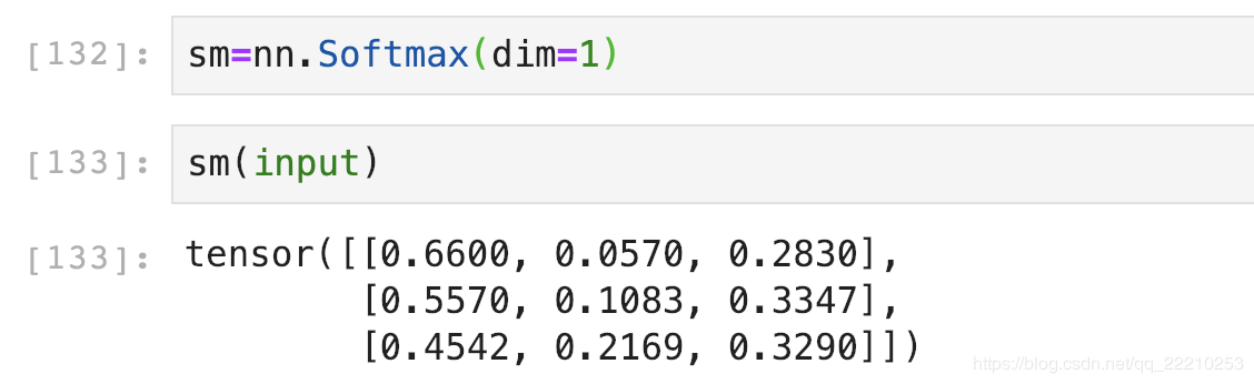
m = nn.Softmax(dim=0)
input = torch.tensor([[2., 2., 2., 2.], [3., 3., 3., 3.]])
print(input.shape)
output = m(input)
print(output)

输出：
torch.Size([2, 4])
tensor([[0.2689, 0.2689, 0.2689, 0.2689],
[0.7311, 0.7311, 0.7311, 0.7311]])

torch.nn.L1Loss

torch.nn.L1Loss(size_average=None, reduce=None, reduction=’mean’)

创建一个标准用来衡量输入x和目标y每个元素之间的均值绝对误差。

如果reduction设置为none， loss如下：

\[l(x, y) = L = \{l_1, ..., l_N\}, l_n = \mid x_n - y_n \mid\]

其中N是batch_size，如果reduction不为none（默认为mean）：

\[l(x, y) = \begin{cases} mean(L), & \text {if reduction = 'mean'} \\ sum(L), & \text {if reduction = 'sum'} \end{cases}\]

Input： (N, *) 其中*表示任意数量额外的维度
Target：(N, *)，与输入的形状相同
Output：标量，如果reduction是none，形状和输入相同

torch.nn.CrossEntropyLoss

NLLLoss

在图片单标签分类时，输入m张图片，输出一个m*N的Tensor，其中N是分类个数。比如输入3张图片，分三类，最后的输出是一个3*3的Tensor，举个例子：

第123行分别是第123张图片的结果，假设第123列分别是猫、狗和猪的分类得分。
可以看出模型认为第123张都更可能是猫。
然后对每一行使用Softmax，这样可以得到每张图片的概率分布。

这里dim的意思是计算Softmax的维度，这里设置dim=1，可以看到每一行的加和为1。比如第一行0.6600+0.0570+0.2830=1。

如果设置dim=0，就是一列的和为1。比如第一列0.2212+0.3050+0.4738=1。
我们这里一张图片是一行，所以dim应该设置为1。
然后对Softmax的结果取自然对数：

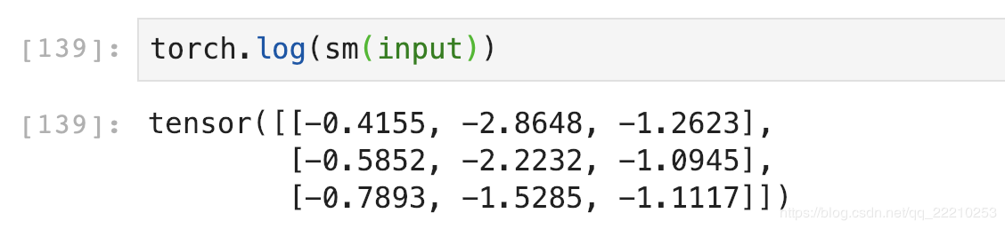
Softmax后的数值都在0~1之间，所以ln之后值域是负无穷到0。
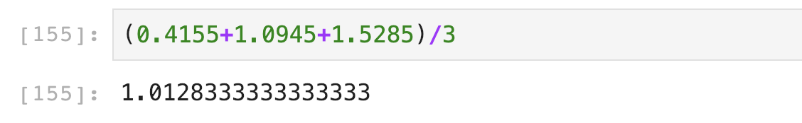
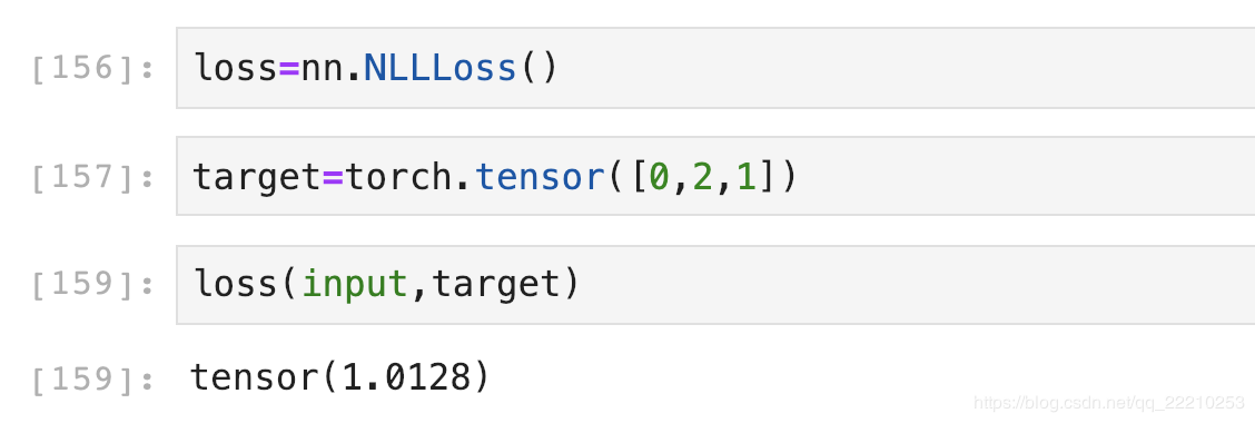
NLLLoss的结果就是把上面的输出与Label对应的那个值拿出来，再去掉负号，再求均值。

假设我们现在Target是[0,2,1]（第一张图片是猫，第二张是猪，第三张是狗）。第一行取第0个元素，第二行取第2个，第三行取第1个，去掉负号，结果是：[0.4155,1.0945,1.5285]。再求个均值，结果是：

下面使用NLLLoss函数验证一下：

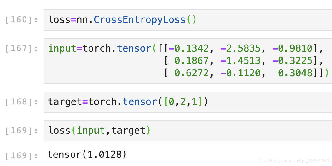
CrossEntropyLoss

CrossEntropyLoss就是把以上Softmax–Log–NLLLoss合并成一步，我们用刚刚随机出来的input直接验证一下结果是不是1.0128：

torch.nn.BCELoss

class torch.nn.BCELoss(weight=None, size_average=True, reduce=True)

weight参数通常默认值是0，如果你的训练样本很不均衡的话，可以设置其值。
size_averaged参数是设置是否取均值，默认是对bach取均值，若设置为False就是对batch求和，这两种情况下损失函数输出的是一个标量
reduce是表示是否size_averaged起作用，默认为True，size_averaged起作用。设置为False，size_averaged不起作用，不求和也不求均值，输出一个向量。

torch.nn.functional.binary_cross_entropy(input, target, weight=None, size_average=None, reduce=None, reduction=’mean’)

input – 任意形状的张量
target – 与输入形状相同的张量
weight (Tensor, 可选的) – 手动重新调整权重, 如果提供, 它重复来匹配输入张量的形状
size_average (bool, 可选的) – 废弃的 (见 reduction). 默认情况下, 批处理中的每个损失元素的平均损失. 注意, 对于某些损失, 每个样本有多个元素. 如果size_average设置为False, 则对每个小批的损失进行汇总. reduce为False时忽略. 默认值: True
reduce (bool, 可选的) – 废弃的 (见 reduction). 默认情况下, 根据size_average, 对每个小批量的观察结果的损失进行平均或求和. 当reduce为False时, 返回每批元素的损失并忽略size_average. 默认值: True
reduction (string__, 可选的) – 指定要应用于输出的reduction：’none’| ‘mean’| ‘sum’. ‘none’：没有reduction, ‘mean’：输出的总和将除以输出中的元素数量 ‘sum’：输出将被求和. 注意：size_average和reduce正在被弃用, 同时, 指定这两个args中的任何一个都将覆盖reduce. 默认值：’mean’, 默认值: ‘mean’

未解决的问题：用BCELoss和binary_cross_entropy，发现输出结果不同

交叉熵的公式：

\[CrossEntropy(Y, \hat Y) = - \sum _c^{N_c}Ylog(\hat Y)\]

上式中$c$为分类编号，$N_c$为所有的分类数量。

在DCGAN中：观察这个公式
$\hat Y$是一个向量， y的值域是经过sigmoid函数激活之后的值域，即(0, 1)
$Y$是一个label组成的向量, 值为0或1。

$J(\theta) = -\sum_{c}^{N_c}Ylog(\hat Y) = 1 * -log(\hat y_{c})$ 在分类任务中, 无论是单分类还是多分类，属于的哪个类别是1.其余是0，将求和函数展开，即可得到等式右侧。

当模型什么东西都没有学到的时候，，模型输出的每个分类的概率是均等的，等于没有做出判断，那么在这种情况下$y_c = \frac{1}{N_c}$, 代入原式可以得到：

\[J(\theta) = -log(\frac{1}{N_c}) = -(log(1) - log(N_c)) = log(N_c)\]

两边同时取$e$，无效学习的情况下： $e^{J(\theta)} \geq N_c$

这个结果说明了，如果模型学到了东西，那么$e^{J(\theta)}$的值应该小于$N_c$：

\[e^{J(\theta)} < N_c\]

torch.nn.BatchNorm2d

class torch.nn.BatchNorm2d(num_features, eps=1e-05, momentum=0.1, affine=True)

num_features：一般输入参数为batch_sizenum_featuresheight*width，即为其中特征的数量
eps：分母中添加的一个值，目的是为了计算的稳定性，默认为：1e-5
momentum：一个用于运行过程中均值和方差的一个估计参数
affine：当设为true时，会给定可以学习的系数矩阵gamma和beta

\[y = \frac{x - mean(x)}{\sqrt{Var(x)} + eps} * \gamma + \beta\]

在卷积神经网络的卷积层之后总会添加BatchNorm2d进行数据的归一化处理，这使得数据在进行Relu之前不会因为数据过大而导致网络性能的不稳定

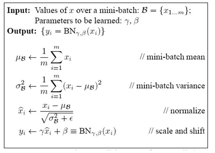
BatchNorm也有参数W和b，这是经过标准化之后的W和b，也就是上图中的Shift和Scale因子$\gamma、\beta$。

torch.nn.InstanceNorm2d

torch.nn.InstanceNorm2d(num_features, eps=1e-05, momentum=0.1, affine=False, track_running_stats=False)

\[y = \frac{x - E[x]}{\sqrt{Var[x] + \epsilon}} * \gamma + \beta\]

num_features – 来自输入尺寸$(N, C, H, W)$的C
affine – 一个布尔类型的数值，如果设置为True，这个模块有可学习的参数，初始化的方式与BatchNorm相同。默认为False。

如果batchsize为1会报错

norm = nn.InstanceNorm2d(3, track_running_stats=True)
x = torch.randn(1, 3, 1, 1)
out = norm(x)
> ValueError: Expected more than 1 value per channel when training, got input size torch.Size([1, 3, 1, 1])

如果单个像素并且batchsize > 1 ， running_var会出问题

norm = nn.InstanceNorm2d(3, track_running_stats=True)
print(norm.running_mean)
> tensor([0., 0., 0.])

print(norm.running_var)
> tensor([1., 1., 1.])

x = torch.randn(8, 3, 1, 1)
out = norm(x)
print(out)
> tensor([[[[0.]],

           [[0.]],

           [[0.]]],
            ...

print(norm.running_mean)
> tensor([ 0.0194, -0.0310, -0.0516])

print(norm.running_var)
> tensor([nan, nan, nan])

如果调用 .eval 解决这个问题

torch.nn.ReflectionPad2d

torch.nn.ReflectionPad2d(padding)

使用输入边界的反射来填充输入Tensor

对于N维的填充，使用torch.nn.functional.pad().

参数：

padding (python:int, tuple)：填充的尺寸，如果是整型，在所有的边界使用同样的填充。如果是一个4-tuple，使用(padding_left, padding_right， padding_top , padding_bottom)

形状：

Input： $(N, C，H_{in}, W_{in})$
Output：$(N, C,H_{out} W_{out})$，其中
$H_{out} = H_{in} + padding_{top} + padding_{bottom}$ $W_{out} = W_{in} + padding_{left} + padding_{right}$

例子：

input = torch.randn(64, 3, 220, 220) # input size
 
# 输入4-tuple
pad = nn.ReflectionPad2d((3, 3, 5, 5))     # left, right, top, bottom
output = pad(input) # size(64, 3, 230, 226)
 
# 输入int
pad = nn.ReflectionPad2d(3)
output = pad(input) # size(64, 3, 226, 226)

增加边界的类型有以下4个类型：

以一行图像数据为例，abcdefgh是原图数据，

是图像边界，为原图加边

aaaaaa abcdefgh hhhhhhh 重复
fedcba abcdefgh hgfedcb 反射
gfedcb abcdefgh gfedcba 反射101，相当于上一行的左右互换
cdefgh abcdefgh abcdefg 外包装
iiiiii abcdefgh iiiiiii with some specified ‘i’ 常量

Note：对于Conv2d中的padding，默认是补0的。

torch.nn.MaxPool2d

torch.nn.MaxPool2d(kernel_size, stride=None, padding=0, dilation=1, return_indices=False, ceil_mode=False)

对几个输入平面组成的输入信号进行二维的最大池化

ceil_mode: 如果为True，使用ceil替代floor计算输出形状

Shape：

Input：$(N, C, H_{in}, W_{in})$
Output：$(N, C, H_{out}, W_{out})$，其中 $H_{out} = \lfloor \frac{H_{in} + 2 * padding[0] - dilation[0] \times (kernel\_size[0] -1) -1}{stride[0]} + 1$

\[W_{out} = \lfloor \frac{W_{in} + 2 * padding[1] - dilation[1] \times (kernel\_size[1] -1) -1}{stride[1]} + 1\]

torch.nn.AvgPool2d

torch.nn.AvgPool2d(kernel_size, stride=None, padding=0, ceil_mode=False, count_include_pad=True, divisor_override=None)

对几个输入平面组成的输入信号进行二维的平均池化

shape：

Input：$(N, C, H_{in}, W_{in})$
Output：$(N, C, H_{out}, W_{out})$

\[H_{out} = \lfloor\frac{H_{in} + 2 \times padding[0] - kernel\_size[0]}{stride[0]} + 1 \rfloor\] \[W_{out} = \lfloor \frac{W_{in} + 2 \times padding[1] - kernel\_size[1]}{stride[1]} + 1 \rfloor\]

kernel_size – the size of the window
stride – the stride of the window. Default value is kernel_size
count_include_pad：当为True的时候，填充的0也将被计算在内

torch.nn.AvgPool3d

torch.nn.AvgPool3d(kernel_size: Union[T, Tuple[T, T, T]], stride: Optional[Union[T, Tuple[T, T, T]]] = None, padding: Union[T, Tuple[T, T, T]] = 0, ceil_mode: bool = False, count_include_pad: bool = True, divisor_override=None)

输入$(N, C, D, H, W)$，输出$(N, C, D_{out}, H_{out}, W_{out})$，核大小$(kD, kH, kW)$

\[D_{out} = \lfloor\frac{D_{in} + 2 \times padding[0] - kernel\_size[0]}{stride[0]} + 1\rfloor\] \[H_{out} = \lfloor\frac{H_{in} + 2 \times padding[1] - kernel\_size[1]}{stride[1]} + 1\rfloor\] \[W_{out} = \lfloor\frac{W_{in} + 2 \times padding[2] - kernel\_size[2]}{stride[2]} + 1\rfloor\]

nn.ConvTranspose2d与nn.Upsample的区别

class torch.nn.Upsample(size=None, scale_factor=None, mode=’nearest’, align_corners=None)

input：(batch_size, channels, Height, Width) output: (batch_size, channels, Height * scale_factor , Width * scale_factor)

class torch.nn.ConvTranspose2d(in_channels, out_channels, kernel_size, stride=1, padding=0, output_padding=0, groups=1, bias=True, dilation=1)

input: (batch_size, channels, Height~in~, Width~in~) output: (batch_size, channels, Height~in~, Width~in~)

\[H_{out} = (H_{in}-1)\times stride[0] - 2 \times padding[0] + kenel\_size[0] + output\_padding[0]\] \[W_{out} = (W_{in}-1)\times stride[1] - 2 \times padding[1] + kenel\_size[1] + output\_padding[1]\]

所以Upsample加上Conv2d实现效果相当于ConvTranspose2d。

这个记住Conv的公式就能反推出来

\[Xout = \frac{X_{in}-F+2P}{S} + 1\]

注意：ConvTranspose2d并不是真正的解卷积操作。

至于要用哪一个，它取决于你的网络设计。如果你确定你需要的是上采样，那么你可以使用nn.Upsample。然而，如果你认为要学习如何上采样而不是硬解码的方式，你可以使用可训练参数的ConvTranspose2d。

class torch.nn.Embedding(num_embeddings, embedding_dim, padding_idx=None, max_norm=None, norm_type=2, scale_grad_by_freq=False, sparse=False)

pytorch中，针对词向量有一个专门的层nn.Embedding，用来实现词与词向量的映射。nn.Embedding具有一个权重，形状是(num_embeddings,embedding_dimension)。例如，输入10个词，每个词用2维向量表征，对应的权重就是一个10x2的矩阵。如果Embedding层的输入形状为NxM（N是batch size,M是序列的长度），则输出的形状是NMembedding_dimension.

nn.PReLU

torch.nn.PReLU(num_parameters: int = 1, init: float = 0.25)

应用于元素级别的函数

\[PReLU(x) = max(0, x) + a * min(0, x)\]

或则

\[PReLU(x) = \begin{cases} x, & if \quad x \geq 0 \\ ax, & otherwise \end{cases}\]

num_parameters (int) – 要学习的a的数目。尽管它的输入是int，这里只有两个值是合法的： 1或者输入的通道数。默认为1。
int(float) - a的初始值。默认为0.25.

ModuleList和Sequential

nn.Sequential

nn.Sequential里面的模块按照顺序进行排列的，所以必须确保前一个模块的输出大小和下一个模块的输入大小是一致的。如下面的例子所示：

#首先导入torch相关包
import torch
import torch.nn as nn
import torch.nn.functional as F
class net_seq(nn.Module):
    def __init__(self):
        super(net2, self).__init__()
        self.seq = nn.Sequential(
                        nn.Conv2d(1,20,5),
                         nn.ReLU(),
                          nn.Conv2d(20,64,5),
                       nn.ReLU()
                       )      
    def forward(self, x):
        return self.seq(x)
net_seq = net_seq()
print(net_seq)
#net_seq(
#  (seq): Sequential(
#    (0): Conv2d(1, 20, kernel_size=(5, 5), stride=(1, 1))
#    (1): ReLU()
#    (2): Conv2d(20, 64, kernel_size=(5, 5), stride=(1, 1))
#    (3): ReLU()
#  )
#)

nn.Sequential中可以使用OrderedDict来指定每个module的名字，而不是采用默认的命名方式(按序号 0,1,2,3…)。例子如下：

from collections import OrderedDict

class net_seq(nn.Module):
    def __init__(self):
        super(net_seq, self).__init__()
        self.seq = nn.Sequential(OrderedDict([
                        ('conv1', nn.Conv2d(1,20,5)),
                         ('relu1', nn.ReLU()),
                          ('conv2', nn.Conv2d(20,64,5)),
                       ('relu2', nn.ReLU())
                       ]))
    def forward(self, x):
        return self.seq(x)
net_seq = net_seq()
print(net_seq)
#net_seq(
#  (seq): Sequential(
#    (conv1): Conv2d(1, 20, kernel_size=(5, 5), stride=(1, 1))
#    (relu1): ReLU()
#    (conv2): Conv2d(20, 64, kernel_size=(5, 5), stride=(1, 1))
#    (relu2): ReLU()
#  )
#)

nn.ModuleList

nn.ModuleList，它是一个储存不同 module，并自动将每个 module 的 parameters 添加到网络之中的容器。你可以把任意 nn.Module 的子类 (比如 nn.Conv2d, nn.Linear 之类的) 加到这个 list 里面，方法和 Python 自带的 list 一样，无非是 extend，append 等操作。但不同于一般的 list，加入到 nn.ModuleList 里面的 module 是会自动注册到整个网络上的，同时 module 的 parameters 也会自动添加到整个网络中。若使用python的list，则会出问题。下面看一个例子：

class net_modlist(nn.Module):
    def __init__(self):
        super(net_modlist, self).__init__()
        self.modlist = nn.ModuleList([
                       nn.Conv2d(1, 20, 5),
                       nn.ReLU(),
                        nn.Conv2d(20, 64, 5),
                        nn.ReLU()
                        ])

    def forward(self, x):
        for m in self.modlist:
            x = m(x)
        return x

net_modlist = net_modlist()
print(net_modlist)
#net_modlist(
#  (modlist): ModuleList(
#    (0): Conv2d(1, 20, kernel_size=(5, 5), stride=(1, 1))
#    (1): ReLU()
#    (2): Conv2d(20, 64, kernel_size=(5, 5), stride=(1, 1))
#    (3): ReLU()
#  )
#)

for param in net_modlist.parameters():
    print(type(param.data), param.size())
#<class 'torch.Tensor'> torch.Size([20, 1, 5, 5])
#<class 'torch.Tensor'> torch.Size([20])
#<class 'torch.Tensor'> torch.Size([64, 20, 5, 5])
#<class 'torch.Tensor'> torch.Size([64])

可以看到，这个网络权重 (weithgs) 和偏置 (bias) 都在这个网络之内。接下来看看另一个作为对比的网络，它使用 Python 自带的 list：

class net_modlist(nn.Module):
    def __init__(self):
        super(net_modlist, self).__init__()
        self.modlist = [
                       nn.Conv2d(1, 20, 5),
                       nn.ReLU(),
                        nn.Conv2d(20, 64, 5),
                        nn.ReLU()
                        ]

    def forward(self, x):
        for m in self.modlist:
            x = m(x)
        return x

net_modlist = net_modlist()
print(net_modlist)
#net_modlist()
for param in net_modlist.parameters():
    print(type(param.data), param.size())
#None

nn.Sequential与nn.ModuleList的区别

不同点1：

nn.Sequential内部实现了forward函数，因此可以不用写forward函数。而nn.ModuleList则没有实现内部forward函数。

对于nn.Sequential：

#例1：这是来自官方文档的例子
seq = nn.Sequential(
          nn.Conv2d(1,20,5),
          nn.ReLU(),
          nn.Conv2d(20,64,5),
          nn.ReLU()
        )
print(seq)
# Sequential(
#   (0): Conv2d(1, 20, kernel_size=(5, 5), stride=(1, 1))
#   (1): ReLU()
#   (2): Conv2d(20, 64, kernel_size=(5, 5), stride=(1, 1))
#   (3): ReLU()
# )

#对上述seq进行输入
input = torch.randn(16, 1, 20, 20)
print(seq(input))
#torch.Size([16, 64, 12, 12])

#例2：或者继承nn.Module类的话，就要写出forward函数
class net1(nn.Module):
    def __init__(self):
        super(net1, self).__init__()
        self.seq = nn.Sequential(
                        nn.Conv2d(1,20,5),
                         nn.ReLU(),
                          nn.Conv2d(20,64,5),
                       nn.ReLU()
                       )      
    def forward(self, x):
        return self.seq(x)

    #注意：按照下面这种利用for循环的方式也是可以得到同样结果的
    #def forward(self, x):
    #    for s in self.seq:
    #        x = s(x)
    #    return x

 #对net1进行输入
input = torch.randn(16, 1, 20, 20)
net1 = net1()
print(net1(input).shape)
#torch.Size([16, 64, 12, 12])

而对于nn.ModuleList：

#例1：若按照下面这么写，则会产生错误
modlist = nn.ModuleList([
         nn.Conv2d(1, 20, 5),
         nn.ReLU(),
         nn.Conv2d(20, 64, 5),
         nn.ReLU()
         ])
print(modlist)
#ModuleList(
#  (0): Conv2d(1, 20, kernel_size=(5, 5), stride=(1, 1))
#  (1): ReLU()
#  (2): Conv2d(20, 64, kernel_size=(5, 5), stride=(1, 1))
#  (3): ReLU()
#)

input = torch.randn(16, 1, 20, 20)
print(modlist(input))
#产生NotImplementedError

#例2：写出forward函数
class net2(nn.Module):
    def __init__(self):
        super(net2, self).__init__()
        self.modlist = nn.ModuleList([
                       nn.Conv2d(1, 20, 5),
                       nn.ReLU(),
                        nn.Conv2d(20, 64, 5),
                        nn.ReLU()
                        ])

    #这里若按照这种写法则会报NotImplementedError错
    #def forward(self, x):
    #    return self.modlist(x)

    #注意：只能按照下面利用for循环的方式
    def forward(self, x):
        for m in self.modlist:
            x = m(x)
        return x

input = torch.randn(16, 1, 20, 20)
net2 = net2()
print(net2(input).shape)
#torch.Size([16, 64, 12, 12])

如果完全直接用 nn.Sequential，确实是可以的，但这么做的代价就是失去了部分灵活性，不能自己去定制 forward 函数里面的内容了。

一般情况下 nn.Sequential 的用法是来组成卷积块 (block)，然后像拼积木一样把不同的 block 拼成整个网络，让代码更简洁，更加结构化。

不同点2：

nn.Sequential可以使用OrderedDict对每层进行命名，上面已经阐述过了；

不同点3：

nn.Sequential里面的模块按照顺序进行排列的，所以必须确保前一个模块的输出大小和下一个模块的输入大小是一致的。而nn.ModuleList 并没有定义一个网络，它只是将不同的模块储存在一起，这些模块之间并没有什么先后顺序可言。见下面代码：

class net3(nn.Module):
    def __init__(self):
        super(net3, self).__init__()
        self.linears = nn.ModuleList([nn.Linear(10,20), nn.Linear(20,30), nn.Linear(5,10)])
    def forward(self, x):
        x = self.linears[2](x)
        x = self.linears[0](x)
        x = self.linears[1](x)

        return x

net3 = net3()
print(net3)
#net3(
#  (linears): ModuleList(
#    (0): Linear(in_features=10, out_features=20, bias=True)
#    (1): Linear(in_features=20, out_features=30, bias=True)
#    (2): Linear(in_features=5, out_features=10, bias=True)
#  )
#)

input = torch.randn(32, 5)
print(net3(input).shape)
#torch.Size([32, 30])

根据 net5 的结果，可以看出来这个 ModuleList 里面的顺序不能决定什么，网络的执行顺序是根据 forward 函数来决定的。若将forward函数中几行代码互换，使输入输出之间的大小不一致，则程序会报错。此外，为了使代码具有更高的可读性，最好把ModuleList和forward中的顺序保持一致。

不同点4：

有的时候网络中有很多相似或者重复的层，我们一般会考虑用 for 循环来创建它们，而不是一行一行地写，比如：

layers = [nn.Linear(10, 10) for i in range(5)]

那么这里我们使用ModuleList：

class net4(nn.Module):
    def __init__(self):
        super(net4, self).__init__()
        layers = [nn.Linear(10, 10) for i in range(5)]
        self.linears = nn.ModuleList(layers)

    def forward(self, x):
        for layer in self.linears:
            x = layer(x)
        return x

net = net4()
print(net)
# net4(
#   (linears): ModuleList(
#     (0): Linear(in_features=10, out_features=10, bias=True)
#     (1): Linear(in_features=10, out_features=10, bias=True)
#     (2): Linear(in_features=10, out_features=10, bias=True)
#   )
# )

torch.nn.Parameter()

可以把这个函数理解为类型转换函数，将一个不可训练的类型Tensor转换成可以训练的类型parameter并将这个parameter绑定到这个module里面(net.parameter()中就有这个绑定的parameter，所以在参数优化的时候可以进行优化的)，所以经过类型转换这个self.v变成了模型的一部分，成为了模型中根据训练可以改动的参数了。使用这个函数的目的也是想让某些变量在学习的过程中不断的修改其值以达到最优化。

打印参数：

for name, param in VGG.named_parameters():
	print(name, '      ', param.size())

关于weight和weight.data

两者数据类型不同

weight的类型是torch.nn.parameter.Parameter

weight的类型是tensor

关于在net中的tensor

如果在网络中随机初始化一个tensor，这个tensor是不属于这个网络的，所以在计算的时候，会出现cuda和cpu不匹配的问题，即如果变量在cuda里，而tensor是在cpu的，两者运算不匹配。

即使net是在cuda中的，也会出现这样问题，所以需要将tensor变成parameter。

class test(nn.Module):
    def __init__(self):
        super().__init__()
        self.noise = nn.Parameter(torch.randn((1 ,3)))
        self.register_parameter('noise', self.noise)

    def forward(self, x):
        out = torch.matmul(x, self.noise)
        return out

x = torch.randn((3, 1)).cuda()
net = test().cuda()
out = net(x)

在不知道batch的情况，可这么做：

class test(nn.Module):
    def __init__(self):
        super().__init__()

    def forward(self, x):
        noise = torch.randn((1, 3)).to(x.device)
        out = torch.matmul(x, noise)
        return out

x = torch.randn((3, 1)).cuda()
net = test().cuda()
out = net(x)

torch.nn.Module

register_parameter(name, param)

给module添加一个参数

可以使用给定名称将参数作为属性访问。

import torch
from torch import nn

class MyModel(nn.Module):
    def __init__(self):
        super(MyModel, self).__init__()
        print('before register:\n', self._parameters, end='\n\n')
        self.register_parameter('my_param1', nn.Parameter(torch.randn(3, 3)))
        print('after register and before nn.Parameter:\n', self._parameters, end='\n\n')

        self.my_param2 = nn.Parameter(torch.randn(2, 2))
        print('after register and nn.Parameter:\n', self._parameters, end='\n\n')

    def forward(self, x):
        return x

mymodel = MyModel()

for k, v in mymodel.named_parameters():
    print(k, v)

程序返回为:

before register:
 OrderedDict()

after register and before nn.Parameter:
 OrderedDict([('my_param1', Parameter containing:
tensor([[-1.3542, -0.4591, -2.0968],
        [-0.4345, -0.9904, -0.9329],
        [ 1.4990, -1.7540, -0.4479]], requires_grad=True))])

after register and nn.Parameter:
 OrderedDict([('my_param1', Parameter containing:
tensor([[-1.3542, -0.4591, -2.0968],
        [-0.4345, -0.9904, -0.9329],
        [ 1.4990, -1.7540, -0.4479]], requires_grad=True)), ('my_param2', Parameter containing:
tensor([[ 1.0205, -1.3145],
        [-1.1108,  0.4288]], requires_grad=True))])

my_param1 Parameter containing:
tensor([[-1.3542, -0.4591, -2.0968],
        [-0.4345, -0.9904, -0.9329],
        [ 1.4990, -1.7540, -0.4479]], requires_grad=True)
my_param2 Parameter containing:
tensor([[ 1.0205, -1.3145],
        [-1.1108,  0.4288]], requires_grad=True)

可以看到register_parameter(name, nn.Parameter())与self.name = nn.Parameter()的功能看起来是相同的。

register_forward_pre_hook()

register_forward_hook中的hooks是文件torch.utils.hooks。RemovableHandle放在该文件中，作用为 “A handle which provides the capability to remove a hook”。register_forward_pre_hook将hook存储到_forward_pre_hooks中。_forward_pre_hooks中的hook在前向传播之前执行。register_forward_hook将hook存储到_forward_hooks中。_forward_hooks中的hook在前向传播计算出结果之后执行。register_backward_hook将hook存储到_backward_hooks中，_backward_hooks中的hook在计算完梯度后执行。

register_buffer(name, tensor)

添加一个buffer给module

这通常用于注册不应被视为模型参数的buffer。比如BatchNorm的running_mean不是一个参数，但是是状态的一部分。

Buffers可以作为属性通过给定名称来获取

定义parameter和buffer都只需要传入Tensor即可。也不需要将其转成gpu,这是因为，当网络进行.cuda时候，会自动将里面的层的参数，buffer等转换成相应的GPU上。
self.register_buffer可以将tensor注册成buffer,在forward中使用self.mybuffer,而不是self.mybuffer_tmp
网络存储时也会将buffer存下，当网络load模型时，会将存储的模型的buffer也进行赋值。
buffer的更新在forward中，optim.step只能更新nn.parameter类型的参数。

torch.nn.modules.utils

torch.nn.modules.utils._pair()

这个函数在官方文档没有找到

经试验

_pair(3)

输出一个tuple：（3， 3）

*_pair(3)

输出迭代器里的内容：3， 3

torch.nn.init

torch.nn.init.normal_(tensor, mean=0.0, std=1.0)

用采样自正态分布的数值填充输入Tensor。

torch.nn.init.xavier_normal_(tensor, gain=1.0)

返回tensor采样自$N(0, std^2)$，其中

\[std = gain \times \sqrt{\frac{2}{fan\_in + fan\_out}}\]

其中fan_in和fan_out是分别权值张量的输入和输出元素数目. 这种初始化同样是为了保证输入输出的方差不变, 在tanh激活函数上有很好的效果，但不适用于ReLU激活函数。

我们来看一下fan_in和fan_out是怎么算的

def _calculate_fan_in_and_fan_out(tensor):
    dimensions = tensor.dim()
    if dimensions < 2:
        raise ValueError("Fan in and fan out can not be computed for tensor with fewer than 2 dimensions")

    num_input_fmaps = tensor.size(1)
    num_output_fmaps = tensor.size(0)
    receptive_field_size = 1
    if tensor.dim() > 2:
        receptive_field_size = tensor[0][0].numel()
    fan_in = num_input_fmaps * receptive_field_size
    fan_out = num_output_fmaps * receptive_field_size

    return fan_in, fan_out

$fan_in = 第二维的维数 \times 第二维之后各维维数乘积$
$fan_out = 第一维的维数 \times 第二维之后各维维数乘积$

t = torch.randn((2, 3, 4, 5))
a, b = _calculate_fan_in_and_fan_out(t)
print(a)
print(b)

60
40

思考：为什么这里的输入对应的第二维，输出对应着第一维？

回答：对于conv2d的参数weight， $(out_channels, \frac{in_channels}{groups}, kH, kW)$

torch.nn.init.kaiming_normal_(tensor, a=0, mode=’fan_in’, nonlinearity=’leaky_relu’)

返回的tensor采样自$N(0, std^2)$

pytorch官网这么写：

\[std = \frac{gain}{fan\_mode}\]

知乎上是这样

\[std = \sqrt{\frac{2}{(1 + a^2) \times fan\_mode}}\]

仔细看了pytorch源代码，它的gain是这么算的

\[\sqrt{\frac{2.0}{1 + negative\_slope^2}}\]

因此是等价的。

a为Relu或Leaky Relu的负半轴斜率
$n_l$为输入的维数

torch.nn.functional as F

上下采样函数–interpolate

根据给定 size 或 scale_factor，上采样或下采样输入数据input.

当前支持 temporal, spatial 和 volumetric 输入数据的上采样，其shape 分别为：3-D, 4-D 和 5-D.

输入数据的形式为：mini-batch x channels x [optional depth] x [optional height] x width.

上采样算法有：nearest, linear(3D-only), bilinear(4D-only), trilinear(5D-only).

参数:

input (Tensor): input tensor
size (int or Tuple[int] or Tuple[int, int] or Tuple[int, int, int]):输出的 spatial 尺寸.
scale_factor (float or Tuple[float]): spatial 尺寸的缩放因子.
mode (string): 上采样算法:nearest, linear, bilinear, trilinear, area. 默认为 nearest.
align_corners (bool, optional): 如果 align_corners=True，则对齐 input 和 output 的角点像素(corner pixels)，保持在角点像素的值. 只会对 mode=linear, bilinear 和 trilinear 有作用. 默认是 False.

最邻近插值：顾名思义，按照距离远近给新像素点赋值，其值与最邻近的像素点值相等。

线性插值：两个像素点间的像素，按照权重线性结合，得到的像素值赋值给新的像素点。

双线性插值

例子：

x = Variable(torch.randn([1, 3, 64, 64]))
y0 = F.interpolate(x, scale_factor=0.5)
y1 = F.interpolate(x, size=[32, 32])

y2 = F.interpolate(x, size=[128, 128], mode="bilinear")

print(y0.shape)
print(y1.shape)
print(y2.shape)

这里注意上采样的时候mode默认是“nearest”，这里指定双线性插值“bilinear” 得到结果

torch.Size([1, 3, 32, 32])
torch.Size([1, 3, 32, 32])
torch.Size([1, 3, 128, 128])

torch.nn.functional.interpolate和torch.nn.upsample的区别:

interpolate是一个函数。

upsample是一个层。

upsample的forward也是用interpolate实现的。

torch.nn.functional.pad

torch.nn.functional.pad(input, pad, mode=’constant’, value=0)

输入tensor的维度从后往前填充。输入的$\lfloor \frac{len(pad)}{2} \rfloor$个维度将会被填充。

torch.nn.functional.conv2d

torch.nn.functional.conv2d(input, weight, bias=None, stride=1, padding=0, dilation=1, groups=1) → Tensor

input – input tensor of shape $(minibatch, in_channels, iH, iW)$
weight – filters of shape $(out_channels, \frac{in_channels}{groups}, kH, kW)$
groups – split input into groups, $in_channels$ should be divisible by the number of groups. Default: 1

torch.nn.functional.linear

torch.nn.functional.linear(input, weight, bias=None)

对输入数据进行线性变换： $y = x A^T + b$

形状：

Input: (N, *, in_features)(N,\∗,in_features)其中 * 意味着任意数量的额外维度
Weight: (out_features, in_features)
Bias: (out_features)
Output: (N, *, out_features)

torch.nn.functional.softmax

torch.nn.functional.softmax(input, dim=None, _stacklevel=3, dtype=None)

Softmax被定义为：

\[Softmax(x_i) = \frac{exp(x_i)}{\sum_j exp(x_j)}\]

它将应用于沿dim的所有切片，并将对其进行重新缩放，以使元素位于[0，1]范围内且总和为1。

torch.nn.functional.binary_cross_entropy_with_logits

torch.nn.functional.binary_cross_entropy_with_logits(input, target, weight=None, size_average=None, reduce=None, reduction='mean', pos_weight=None)

计算目标和输出的二分交叉熵的对数。

参数：

weight (Tensor, optional) – 一个手动缩放权重，如果匹配输入tensor形状
size_average (bool, optional) – Deprecated (see reduction).
reduce (bool, optional) – Deprecated (see reduction).

reduction (string, optional) – 应用到输出的指定规约： ‘none’

‘ mean’

‘sum’。 Note : size_average 和 reduce 的处理已经弃用，同时，如果指定这两个参数将会覆盖掉 reduction. 默认 ‘mean’。

pos_weight (Tensor, optional) – 正样本的权重。必须是一个长度和类数量相等的向量。

torch.nn.utils.spectral_norm

对给定模块的参数使用谱规范化

\[W_{SN} = \frac{W}{\sigma(W)}, \sigma(W) = \max_{h:h \neq 0} \frac{\|Wh\|_2}{\|h\|_2}\]

谱规范化通过谱范数缩放权重稳定生成对抗网络中的判决器的训练。

torch.nn.RNN

torch.nn.RNN(*args, **kwargs)

torch.nn.GRU

torch.nn.GRU(*args, **kwargs)

Outputs: output, h_n

output的形状(seq_len, batch, num_directions * hidden_size)：每个时间步 $t$ GRU最后一层输出特征 $h_t$。如果 torch.nn.utils.rnn.PackedSequence 作为输入给定，输出将也是一个packed的序列。对于unpacked的情况，使用 output.view(seq_len, batch, num_directions, hidden_size) 分开方向，前向后反向分别是0和1。相似地，方向在packed的情况可以被分开。
h_n的形状(num_layers * num_directions, batch, hidden_size)：时间步 $t = seq_len$的隐藏状态，层数可以使用 h_n.view(num_layers, num_directions, batch, hidden_size)分开。

torch.nn.Dropout

torch.nn.Dropout(p: float = 0.5, inplace: bool = False)

p：元素归零的概率，默认0.5
inplace：会覆盖掉原变量，可以节省显存。

torch.autograd

torch.autograd.grad

torch.autograd.grad(outputs, inputs, grad_outputs=None, retain_graph=None, create_graph=False, only_inputs=True, allow_unused=False)

计算 outputs 对 inputs 的梯度和。

如果 only_inputs 为 True, 函数将会返回指定输入的梯度列表。如果为 False，梯度将会保留至被计算，并且将会累计到 .grad 属性。

outputs (sequence of Tensor) – outputs 对 inputs 求导
inputs (sequence of Tensor) – outputs 对 inputs 求导
grad_outputs (sequence of Tensor) – Jacobian-vector 内积的向量。对于标量张量和不需要梯度的张量为None值。如果None值可被所有 grad_tensors 接受，那么这个参数是可选的。

requires_grad和torch.no_grad

requires_grad=True的变量的运算结果的requires_grad也为True，这意味着前向传播时会计算并保留该变量的梯度，一般情况下，训练的数据一开始requires_grad是不为True的，但是和参数（weight, bias）等需要requies_grad=True（因为需要优化参数）进行运算后的结果是requires_grad=True的，因为需要它们反向传播提供梯度来更新参数(weight, bias等)。

with torch.no_grad：意味着接下来的运算只进行inference，不保留梯度，requires_grad=False。这样可能会导致梯度链断掉，只有在你确定这部分运算的梯度用不到时，才使用它。使用它可以节省显存，因为不保留梯度。

class test_net(nn.Module):
    def __init__(self):
        super().__init__()
        self.weight  = nn.Parameter(torch.tensor([[2., 2.], [2., 2.]]), requires_grad=True)
        

    def forward(self, input):
        out = self.weight.matmul(input)

        return out

net1 = test_net()
net1.eval()
net2 = test_net()
# op1 = optimizer.Adam(net1.parameters(), 0.001)
op2 = optimizer.Adam(net2.parameters(), 0.001)

#op1.zero_grad()
op2.zero_grad()

t = torch.tensor([[1., 2.], [3, 4]])

# with torch.no_grad():
#     out = net1(t)

out = net1(t)

out = net2(out).mean()

print(out)

out.backward()
# op1.step()
op2.step()

print(net1.weight)
print(net2.weight)

结果：\

tensor(40., grad_fn=<MeanBackward0>)
Parameter containing:
tensor([[2., 2.],
[2., 2.]], requires_grad=True)
Parameter containing:
tensor([[1.9990, 1.9990],
[1.9990, 1.9990]], requires_grad=True)

此时使用不使用with torch.no_grad()运算结果没有差别，但是会缓存计算的梯度。

requires_grad=False，参数不会更新，不需要在优化器参数中特意指定

class test_net(nn.Module):
    def __init__(self):
        super().__init__()
        self.weight  = nn.Parameter(torch.tensor([[2., 2.], [2., 2.]]), requires_grad=True)
        self.weight1 = nn.Parameter(torch.tensor([[2., 2.], [2., 2.]]), requires_grad=False)
        

    def forward(self, input):
        out = self.weight.matmul(input)
        out = self.weight1.matmul(out)

        return out

import torch.optim as optimizer

net1 = test_net()
net1.eval()
net2 = test_net()
# op1 = optimizer.Adam(net1.parameters(), 0.001)
op2 = optimizer.Adam(net2.parameters(), 0.001)

#op1.zero_grad()
op2.zero_grad()

t = torch.tensor([[1., 2.], [3, 4]])

# with torch.no_grad():
#     out = net1(t)

out = net1(t)

out = net2(out).mean()

print(out)

out.backward()
# op1.step()
op2.step()

print(net1.weight)
print(net2.weight)

print(net1.weight1)
print(net2.weight1)

输出：
Parameter containing:
tensor([[2., 2.],
[2., 2.]], requires_grad=True)
Parameter containing:
tensor([[1.9990, 1.9990],
[1.9990, 1.9990]], requires_grad=True)
Parameter containing:
tensor([[2., 2.],
[2., 2.]])
Parameter containing:
tensor([[2., 2.],
[2., 2.]])

model.train和model.eval

model.eval()和torch.no_grads不同，并不是预测时不提供梯度，而是使drop_out和BatchNorm等失活。

只有将参数添加进optimizer，参数才会被优化。

也就是说，即便是开启eval模式，将参数送入optimizer，参数也会被更新。

class test_net(nn.Module):
    def __init__(self):
        super().__init__()
        self.weight  = nn.Parameter(torch.tensor([[2., 2.], [2., 2.]]), requires_grad=True)
        

    def forward(self, input):
        out = self.weight.matmul(input)

        return out

net1 = test_net()
net1.eval()
net2 = test_net()
op1 = optimizer.Adam(net1.parameters(), 0.001)
op2 = optimizer.Adam(net2.parameters(), 0.001)

op1.zero_grad()
op2.zero_grad()

t = torch.tensor([[1., 2.], [3, 4]])

# with torch.no_grad():
#     out = net1(t)

out = net1(t)

out = net2(out).mean()

print(out)

out.backward()
op1.step()
op2.step()

print(net1.weight)
print(net2.weight)

结果：
tensor(40., grad_fn=<MeanBackward0>)
Parameter containing:
tensor([[1.9990, 1.9990],
[1.9990, 1.9990]], requires_grad=True)
Parameter containing:
tensor([[1.9990, 1.9990],
[1.9990, 1.9990]], requires_grad=True)

此时，虽然开启了eval模式，但是把参数送入了优化器，反向传播时，仍然会更新网络的权重。

使用with torch.no_grad()时，权重不会更新。

总结：

当网络的参数没有送入优化器时，使用torch.no_grad与否不会影响权重，但是使用会节省显存。

当网络的参数送入了优化器时，不管是eval模式还是train模式，都会更新参数，只有使用torch.no_grad时（即requires_grad=False），不会更新参数。

求导

1) 想使x支持求导，必须让x为浮点类型，也就是我们给初始值的时候要加个点：“.”。不然的话，就会报错。即，不能定义[1,2,3]，而应该定义成[1.,2.,3.]，前者是整数，后者才是浮点数。

2) 求导，只能是【标量】对标量，或者【标量】对向量/矩阵求导！

retain_graph

错误解释：在更新D网络时的loss反向传播过程中使用了retain_graph=True，目的为是为保留该过程中计算的梯度，后续G网络更新时使用；

正解：如果设置为False，计算图中的中间变量在计算完后就会被释放。

具体看一个例子理解：

假设一个我们有一个输入x，$y = x^2$, $z = y \times 4$，然后我们有两个输出，一个output_1 = z.mean()，另一个output_2 = z.sum()。然后我们对两个output执行backward。

import torch
x = torch.randn((1,4),dtype=torch.float32,requires_grad=True) y = x ** 2 4 z = y * 4 
print(x) 
print(y) 
print(z) 
loss1 = z.mean() 
loss2 = z.sum() 
print(loss1,loss2) 
loss1.backward()
loss2 = z.sum() 
print(loss1,loss2) 
loss1.backward()

这个代码执行正常，但是执行完中间变量都free了，所以下一个出现了问题 12 print(loss1,loss2) 13 loss2.backward() # 这时会引发错误程序正常执行到第12行，所有的变量正常保存。但是在第13行报错：

RuntimeError: Trying to backward through the graph a second time, but the buffers have already been freed. Specify retain_graph=True when calling backward the first time.

分析：计算节点数值保存了，但是计算图x-y-z结构被释放了，而计算loss2的backward仍然试图利用x-y-z的结构，因此会报错。

因此需要retain_graph参数为True去保留中间参数从而两个loss的backward()不会相互影响。

关于retain_graph的验证

网络结构：

class E(nn.Module):
    def __init__(self):
        super().__init__()
        self.weight = nn.Parameter(torch.tensor([[2., 2.], [1., 1.]]), requires_grad=True)

    def forward(self, input):
        out = torch.mm(input, self.weight)
        return out
    
class D(nn.Module):
    def __init__(self):
        super().__init__()
        self.weight = nn.Parameter(torch.tensor([[3., 3.], [4., 4.]]), requires_grad=True)

    def forward(self, input):
        out = torch.mm(input, self.weight)

        return out

计算准备：

t = torch.tensor([[1., 2.], [3., 4.]])

target = torch.tensor([[1., 1.], [1., 1.]])

netE = E()
netD = D()

optim_E = torch.optim.Adam(netE.parameters(), 0.01, [0, 0.999])
optim_D = torch.optim.Adam(netD.parameters(), 0.01, [0, 0.999])

crtic = nn.L1Loss()

t1 = netE(t)
t2 = netD(t1)

loss = crtic(t2, target)

如果以这样的形式使用计算梯度：

optim_E.zero_grad()
loss.backward()
optim_E.step()


for name, parms in netE.named_parameters():
    print('E-->name:', name, '-->grad_requirs:', parms.requires_grad, '--weight', torch.mean(parms.data), ' -->grad_value:', torch.mean(parms.grad))

optim_D.zero_grad()
loss.backward()
optim_D.step()


for name, parms in netD.named_parameters():
    print('D-->name:', name, '-->grad_requirs:', parms.requires_grad, '--weight', torch.mean(parms.data), ' -->grad_value:', torch.mean(parms.grad))

报错，因为在第一次backward之后，计算图就已经被释放掉了，而第二处的backward仍要使用已经被释放掉的计算图，若在第一次backward加上retain_graph，则不会释放计算图

如果以下面的方法计算梯度：

optim_E.zero_grad()
loss.backward()
optim_E.step()


for name, parms in netE.named_parameters():
    print('E-->name:', name, '-->grad_requirs:', parms.requires_grad, '--weight', torch.mean(parms.data), ' -->grad_value:', torch.mean(parms.grad))

optim_D.zero_grad()

optim_D.step()


for name, parms in netD.named_parameters():
    print('D-->name:', name, '-->grad_requirs:', parms.requires_grad, '--weight', torch.mean(parms.data), ' -->grad_value:', torch.mean(parms.grad))

也就是去掉第二次的backward，计算出的D梯度为0，因为前面手动将D的梯度清零了。

如果使用下面的方法计算梯度：

optim_D.zero_grad()
optim_E.zero_grad()
loss.backward()
optim_E.step()
optim_D.step()


for name, parms in netE.named_parameters():
    print('E-->name:', name, '-->grad_requirs:', parms.requires_grad, '--weight', torch.mean(parms.data), ' -->grad_value:', torch.mean(parms.grad))


for name, parms in netD.named_parameters():
    print('D-->name:', name, '-->grad_requirs:', parms.requires_grad, '--weight', torch.mean(parms.data), ' -->grad_value:', torch.mean(parms.grad))

计算结果与加了retain_graph相同，因为第一次backward的时候，已经把E和D的梯度都算出来了。

torch.autograd.Function

记录操作历史并且为求偏导操作定义公式。

每个执行在Tensor s上的操作创建一个新的函数对象，这个函数对象执行计算并记录它的发生。这个历史以DAG的形式被保存下来，边表示数据的流动（$input \leftarrow output$）。然后，当被调用backward时，图将会以拓扑结构的顺序实行，通过每个函数对象调用backward()方法，并且将返回的梯度传递到下一个Fuction s。

通常地，用户使用fuctions的唯一方式时创建子类并定义新的操作。这是拓展torch.autograd的推荐方式。

每个函数对象只被使用一次（在前向传播时）

Examples:

>>> class Exp(Function):
>>>
>>>     @staticmethod
>>>     def forward(ctx, i):
>>>         result = i.exp()
>>>         ctx.save_for_backward(result)
>>>         return result
>>>
>>>     @staticmethod
>>>     def backward(ctx, grad_output):
>>>         result, = ctx.saved_tensors
>>>         return grad_output * result

STATIC backward(ctx, *grad_outputs)

为求偏导操作定义一个公式。

这个函数将被所有子类重写。

它必须以ctx作为第一个参数，紧接着的是和forward()返回的输出一样多的参数，并且它应该返回与forward()的输入一样多的Tensor。每个参数是给定输出的梯度，每个返回值应该是相关输入的梯度。

context被用来检索保存在前向传播期间的Tensor。它应该有一属性ctx.needs_input_grad是布尔类型的元组，表示是否每个输入需要梯度， backward()会使ctx.need_input_grad[0] = True, 如果forward的第一个输入需要计算梯度。

STATIC forward(ctx, *args, **kwargs)

执行操作

这个函数被所有子类重写

它必须接受一个context ctx作为第一个参数，紧接着是任意数量的参数(tensor或着其他类型)

context可以被用来存储tensor，这些tensor可以在backward期间被检索到。

torch.optim

Per-parameter options

Optimizer 支持指定每个参数的操作。为了达成这个目的，不是传入一个可迭代的变量，而是传入一个可迭代的dict。

例如，当你想要指定某一层的学习率时，这非常有用：

optim.SGD([
                {'params': model.base.parameters()},
                {'params': model.classifier.parameters(), 'lr': 1e-3}
            ], lr=1e-2, momentum=0.9)

这意味着模型的基础参数将使用1e-2的默认学习率， model.classifier的参数将会使用1e-3的学习率，动量0.9将被用在所有参数中。

add_param_group

add_param_group(param_group)

给优化器的参数组增加一个参数组

当对预训练的网络进行微调时，这很有用，因为可以使冻结的层成为可训练的，并随着训练的进行而添加到优化器中。

param_group (dict) – 指定什么样的Tensor应该随着该组被优化
optimization options. (specific)

torch.distribute

如何使用分布式单机多卡

初始化

配置可用GPU

os.environ['CUDA_VISIBLE_DEVICES'] = "0, 1, 2, 3"

要使用argparse配置local_rank参数

parser = argparse.ArgumentParser()
parser.add_argument('--local_rank', default=-1, type=int,
                    help='node rank for distributed training')
args = parser.parse_args()
					

初始化通信协议

torch.distributed.init_process_group(backend='nccl')

设定当前进程使用的 GPU

torch.cuda.set_device(args.local_rank)

数据集

使用 DistributedSampler 对数据集进行划分，它能帮助我们将每个 batch 划分成几个 partition，在当前进程中只需要获取和 rank 对应的那个 partition 进行训练：

train_sampler = torch.utils.data.distributed.DistributedSampler(train_dataset)

train_loader = torch.utils.data.DataLoader(train_dataset, batch_size=..., sampler=train_sampler)

读取数据后，将数据载入cuda

Xs = Xs.cuda(self.config.local_rank, non_blocking=True)

模型

使用 DistributedDataParallel 包装模型，它能帮助我们为不同 GPU 上求得的梯度进行 all reduce（即汇总不同 GPU 计算所得的梯度，并同步计算结果）。all reduce 后不同 GPU 中模型的梯度均为 all reduce 之前各 GPU 梯度的均值：

model = torch.nn.parallel.DistributedDataParallel(model, device_ids=[args.local_rank])

有的时候你会发现另外几个进程会在0卡上占一部分显存，导致0卡显存出现瓶颈，可能会导致cuda-out-of-memory 错误

当你用

checkpoint = torch.load("checkpoint.pth")
model.load_state_dict(checkpoint["state_dict"])

这样load一个 pretrained model 的时候，torch.load() 会默认把load进来的数据放到0卡上，这样4个进程全部会在0卡占用一部分显存。

解决的方法也很简单，就是把load进来的数据map到cpu上：

checkpoint = torch.load("checkpoint.pth", map_location=torch.device('cpu'))
model.load_state_dict(checkpoint["state_dict"])

启动

python -m torch.distributed.launch --nproc_per_node=4 main.py

其中–nproc_per_node表示gpu数。

BN的问题

调用DDP有类似version counter不对的inplace操作错误，可能是包装的module有register buffer，设置下DDP的参数broadcast_buffers=False。

BN的runing mean和var也是不要求导的buffer。参考：Inplace error if DistributedDataParallel module that contains a buffer is called twice · Issue #22095 · pytorch/pytorch

RuntimeError: one of the variables needed for gradient computation has been modified by an inplace operation: [torch.cuda.FloatTensor [1, 32]] is at version 3; expected version 2 instead

模型的保存与加载

torch.utils.checkpoint

torch.utils.checkpoint.checkpoint(function, *args, use_reentrant=True, **kwargs)

在反向传播中，会检索保存的输入和函数，然后在函数上再次计算前向传播，现在跟踪中间激活，然后使用这些激活值计算梯度。

函数的输出可以包含非张量值，梯度记录只对张量值进行。注意，如果输出由由张量组成的嵌套结构(例如:自定义对象、列表、字典等)组成，这些嵌套在自定义结构中的张量将不会被视为 autograd 的一部分。

torch.utils.data

random_split

torch.utils.data.random_split(dataset, lengths, generator=<torch._C.Generator object>)

随机将一个数据集分割成给定长度的不重叠的新数据集。可选地固定生成器以获得可重现的结果。

例如：

>>> random_split(range(10), [3, 7], generator=torch.Generator().manual_seed(42))

参数：

dataset (Dataset) – 要拆分的数据集。
lengths (sequence) – 要产生的分片的长度。
generator (Generator) – 生成器用于随机排列。

map-style 和 iterable-style(from ChatGPT)

PyTorch 是一个开源的深度学习框架，它提供了两种不同的风格来处理数据：map-style 和 iterable-style。

map-style 数据处理方式是将数据集作为一个整体来处理，并且可以对整个数据集进行并行处理。这种方式通常用于处理较大的数据集，因为它可以有效利用多核处理器的优势来提高处理速度。

iterable-style 数据处理方式是将数据集作为一个可迭代的序列来处理，每次迭代只处理数据集中的一个样本。这种方式通常用于处理较小的数据集，因为它可以避免将整个数据集加载到内存中。

两种方式都可以用于深度学习模型的训练和评估，但是在实际使用中，选择哪种方式取决于数据集的大小和处理目标。

torch.nn.utils.rnn

PackedSequence

RNN 模块接收

pack_padded_sequence

pad_packed_sequence

Torch.Profiler

torch.profiler.profile

torch.profiler.profile(*, activities=None, schedule=None, on_trace_ready=None, record_shapes=False, profile_memory=False, with_stack=False, with_flops=False, use_cuda=None)

Profiler context manager.

Args：

activities - 使用 profiling 的活动组 (CPU, CUDA)，支持的值： torch.profiler.ProfilerActivity.CPU, torch.profiler.ProfilerActivity.CUDA; 默认值： ProfilerActivity.CPU 和 ProfilerActivity.CUDA(如果可用的话)；
schedule - 可调用的，以step (int)作为单个参数并返回 ProfilerAction 值，它在每一步执行指定的 profiler action。
on_trace_ready：在 profiling期间，当 schedule 返回 ProfilerAction.RECORD_AND_SAVE 时，在每一步调用
record_shapes：保存有关运算符输入形状的信息
with_stack：记录操作的源信息(文件和行号)
with_flops：利用公式估计特定算子(矩阵乘法和2D卷积)的FLOPS
use_cuda ：已废弃，使用 activities

注意：

使用 torch.profiler.schedule 生成可调用的schedule。当profiling长期的训练工作时，非默认的 schedules 是有用的，并且允许用户得到在训练期间不同迭代的多个traces。默认schedule只是在 context manager 期间连续记录所有事件。

注意：

使用 torch.profiler.tensorboard_trace_handler 生成用于 Tensorboard 的结果文件。 on_trace_ready=torch.profiler.tensorboard_trace_handler(dir_name), 在 profiling 之后，结果文件在指定的文件夹中。使用命令：
tensorboard --log_dir=dir_name
在 Tensorboard 中查看结果。

注意：

启用 shape 和 stack tracing 将产生额外的开销。

例子：

with torch.profiler.profile(
    activities=[
        torch.profiler.ProfilerActivity.CPU,
        torch.profiler.ProfilerActivity.CUDA]
) as p:
    code_to_profile()
print(p.key_averages().table(
    sort_by="self_cuda_time_total", row_limit=-1))

使用 profiler 的 schedule, on_trace_ready 和 step 函数

# Non-default profiler schedule allows user to turn profiler on and off
# on different iterations of the training loop;
# trace_handler is called every time a new trace becomes available
def trace_handler(prof):
    print(prof.key_averages().table(
        sort_by="self_cuda_time_total", row_limit=-1))
    # prof.export_chrome_trace("/tmp/test_trace_" + str(prof.step_num) + ".json")

with torch.profiler.profile(
    activities=[
        torch.profiler.ProfilerActivity.CPU,
        torch.profiler.ProfilerActivity.CUDA],

    # In this example with wait=1, warmup=1, active=2,
    # profiler will skip the first step/iteration,
    # start warming up on the second, record
    # the third and the forth iterations,
    # after which the trace will become available
    # and on_trace_ready (when set) is called;
    # the cycle repeats starting with the next step

    schedule=torch.profiler.schedule(
        wait=1,
        warmup=1,
        active=2),
    on_trace_ready=trace_handler
    # on_trace_ready=torch.profiler.tensorboard_trace_handler('./log')
    # used when outputting for tensorboard
    ) as p:
        for iter in range(N):
            code_iteration_to_profile(iter)
            # send a signal to the profiler that the next iteration has started
            p.step()

events()

返回未聚合的 profiler events 列表，用于 trace callback 中或 profiling 完成后

export_chrome_trace(path)

导出收集的 trace 以Chrome JSON格式。

export_stacks(path, metric=’self_cpu_time_total’)

以一种适合于可视化的形式保存 stack traces。

参数：

path：保存 stacks 文件的位置
metric：使用的metric： “self_cpu_time_total” 和 “self_cuda_time_total”

Example of using FlameGraph tool:

git clone https://github.com/brendangregg/FlameGraph

cd FlameGraph

./flamegraph.pl –title “CPU time” –countname “us.” profiler.stacks > perf_viz.svg

key_averages(group_by_input_shape=False, group_by_stack_n=0)

Averages events，根据操作符名称和(可选的)输入形状和堆栈将它们分组。注意：使用 shape/stack 函数确保当创建 profiler context manager 时设置 record_shapes/with_stack 。

step()

给 profiler 发送信号，告知它下一步的profiling已经开始了。

torch.profiler.schedule

torch.profiler.schedule(*, wait, warmup, active, repeat=0)

返回一个可调用对象，可作为profiler的 schedule 参数。profiler 将会等待 wait 步，然后为下一个 warmup 步做 warmup，然后为下一个 active 步做active recording 然后从下个步开始循环。循环的次数通过 repeat 参数指定。当参数的值为0时，循环将持续不断，直到profiling完成。

torch.profiler.tensorboard_trace_handler

torch.profiler.tensorboard_trace_handler(dir_name, worker_name=None)

输出 tracing 文件到 dir_name 文件夹，然后哪个文件夹可以直接作为 logdir 分发到 Tensorboard。 worker_name 在分布式场景下对于每个worker应该是不同的，它默认被设置为 ‘[hostname]_[pid]‘。

Dataset & Dataloader

图像预处理

class torchvision.transforms.Compose(transforms) 将多个transform组合起来使用。 transforms：由transform构成的列表.

transforms.Compose([
     transforms.CenterCrop(10),
     transforms.ToTensor(),
 ])

transforms.Resize(img_size)

这个函数只会将行和列相等的矩阵拉成img_size，如果图片长宽不等会出错。

Dataset

torch.utils.data.Dataset是一个抽象类，用户想要加载自定义的数据只需要继承这个类，并且覆写其中的两个方法即可：

__len__:实现len(dataset)返回整个数据集的大小。
__getitem__用来获取一些索引的数据，使dataset[i]返回数据集中第i个样本。

torchvision.datasets

dset.ImageFolder(root=”root folder path”, [transform, target_transform])

Dataloader

class torch.utils.data.DataLoader(dataset, batch_size=1, shuffle=False, sampler=None, num_workers=0, collate_fn=<function default_collate>, pin_memory=False, drop_last=False)

组合数据集和采样器，并在给定的数据集上提供迭代器。

dataset (Dataset)：来自加载数据的数据集
batch_size (python:int, optional)：一批加载多少个样本（默认为1）
shuffle (bool, optional) ：每个epoch重新打乱数据
sampler (Sampler, optional) ：定义从数据集中的采样策略，如果指定，shuffle必须为False
batch_sampler (Sampler, optional)：类似于sampler，但一次返回一批索引。与batch_size，shuffle，sampler和drop_last互斥。
num_workers (python:int, optional)：多少个子进程用于数据加载。 0表示将在主进程中加载数据。（默认值：0）
drop_last (bool, optional) ：如果数据集大小不能被批量大小整除，则设置为True以删除最后一个不完整的批量。如果为False并且数据集的大小不能被批次大小整除，则最后一批将较小。（默认值：False）

从dataloader加载出来的数据就是Tensor

自建数据集

import torch
from torchvision import transforms, datasets
from torch.utils import data

from PIL import Image

import glob

class Dataset(data.Dataset):
    def __init__(self, root, transforms=None):
        self.imgs = glob.glob(root+'/*')
        self.trans = transforms
        

    def __getitem__(self, index):
        x_path = self.imgs[index]
        img_x = Image.open(x_path)
        img_x = self.trans(img_x)

        return img_x

    def __len__(self):
        return len(self.imgs)

class Data_Loader():
    def __init__(self, img_size, img_path, batch_size):
        super(Data_Loader, self).__init__()
        self.img_size = img_size
        self.img_path = img_path
        self.batch_size = batch_size
        self.trans = transforms.Compose(
            [
                transforms.Resize((self.img_size, self.img_size)), 
                transforms.ToTensor(),
                transforms.Normalize([0.5, 0.5, 0.5], [0.5, 0.5, 0.5])
            ]
        )
        self.dataset = Dataset(img_path, self.trans)
        

    def loader(self):
        loader = torch.utils.data.DataLoader(
            self.dataset,
            batch_size=self.batch_size,
            shuffle=True,
            num_workers=0,
            drop_last=True
        )

        return loader

class Dataset(Dataset):
    def __init__(self, root, transforms=None):
        # 用来存放数据路径和标签
        self.imgs = []
        # 制作index和class的映射
        self.label_map = {}
        i = 0
        # 先把各个类的文件夹找到
        paths = sorted(glob.glob(root + "/*"))
        for path in paths:

            self.label_map[path.split("/")[-1]] = i
            single_class = glob.glob(path + "/*")
            # 读取每一个class的文件夹下的数据
            for img in single_class:
                self.imgs.append((img, i))

            i += 1
        self.trans = transforms
        print(len(self.imgs))
        

    def __getitem__(self, index):
        img_path, label = self.imgs[index]
        img = Image.open(img_path)
        if self.trans:
            img = self.trans(img)

        return (img, label)

    def __len__(self):
        return len(self.imgs)

def ImageLoader(root, img_size, batch_size, train=True):
    if train:
        train_trans = transforms.Compose(
            [
                transforms.RandomResizedCrop((img_size, img_size)),
                transforms.ToTensor(),
                # transforms.Normalize([0.5, 0.5, 0.5], [0.5, 0.5, 0.5])
            ]
        )
        dataset = Dataset(root, train_trans)
        loader = DataLoader(
            dataset,
            batch_size=batch_size,
            shuffle=True,
            num_workers=0,
            drop_last=True
        )
    else:
        test_trans = transforms.Compose(
            [
                # transforms.Resize((img_size, img_size)),
                transforms.ToTensor(),
                # transforms.Normalize([0.5, 0.5, 0.5], [0.5, 0.5, 0.5])
            ]
        )
        dataset = Dataset(root, test_trans)
        loader = DataLoader(
            dataset,
            batch_size=batch_size,
            shuffle=False,
            num_workers=0,
            drop_last=False
        )

    return loader

torchvision

transform

torchvision.transforms.ColorJitter

torchvision.transforms.ColorJitter(brightness=0, contrast=0, saturation=0, hue=0)

随机改变图像的亮度、对比度和饱和度。

brightness(python:float or tuple of python:float (min, max))：调整多少亮度。brightness_factor应该均匀地分布在[max(0, 1-brightness), 1+brightness]或者给定[min, max]。它应该是一个非负数。
contrast(python:float or tuple of python:float (min, max))：调整多少对比度。contrast_factor应该均匀地分布在[max(0, 1-contrast), 1+contrast]或者给定[min, max]。它应该是一个非负数。
saturation (python:float or tuple of python:float (min, max))：调整多少饱和度。saturation_factor应该均匀地分布在[max(0, 1-saturation), 1+saturation]或者给定[min, max]。它应该是一个非负数。
hue (python:float or tuple of python:float (min, max))：调整多少色调。hue_factor应该均匀地分布在[-hue， hue]或者给定[min, max]。它应该0 <= hue <= 0.5 或者 -0.5 <= min <= max <= 0.5。

torchvision.transforms.Normalize

torchvision.transforms.Normalize(mean, std, inplace=False)

pytorch使用的预训练模型搭配的数据必须是：

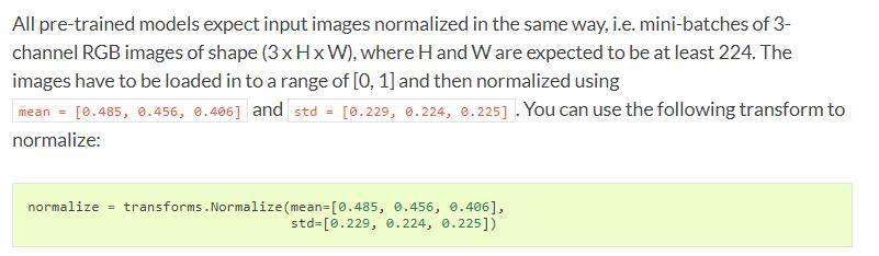
也就是3通道RGB图像(3 x H x W)，而且高和宽最好不低于224(因为拿来做预训练的模型大小就是224 x 224),并且图像数据大小的范围为[0-1]，使用mean和std去Normalize。

为什么这样说官方也说了，因为所有的预训练模型是使用经过normal后的数据得到的，所以我们输入的数据也必须经过格式化，否则很容易出现损失爆炸。

torchvision.transforms.Resize

torchvision.transforms.Resize(size, interpolation=2)

size : 获取输出图像的大小
interpolation : 插值，默认的 PIL.Image.BILINEAR，一共有4中的插值方法
PIL.Image.BICUBIC，PIL.Image.LANCZOS，PIL.Image.BILINEAR，PIL.Image.NEAREST

注意：transform中，Resize要用在ToTensor之前，Normalize要用在ToTensor之后。

torchvision.transforms.ToTensor

torchvision.transforms.ToTensor

将PIL图片或者numpy.ndarray转成一个Tensor

将范围[0, 255]的PIL图像或者形状为$(H \times W \times C)$的numpy.ndarray转化为一个值从[0.0, 1.0]的，形状为$(C \times H \times W)$的torch.FloatTensor。PIL图像属于（L, LA, P, I, F, RGB, YCbCr, RGBA, CMYK, 1）中的一种或者numpy.ndarray的类型为dtype = np.uint8。

torchvision.transforms.ToPILImage

torchvision.transforms.ToPILImage(mode=None)

将一个Tensor或者ndarray转化为PIL图片

保留值范围的情况下把一个形状为$C \times H \times W$或者一个形状为$H \times W \times C$的numpy ndarray。

mode (PIL.Image mode) –

如果输入是四个通道， mode是RGBA
如果输入是三个通道，mode是RGB
如果输入是两个通道， mode是LA
如果输入是一个通道，mode由数据类型决定(例如int, float, short)

经过测试，当通道大于4时，会转化为3通道的图像

源代码：

else:
        permitted_3_channel_modes = ['RGB', 'YCbCr', 'HSV']
        if mode is not None and mode not in permitted_3_channel_modes:
            raise ValueError("Only modes {} are supported for 3D inputs".format(permitted_3_channel_modes))
        if mode is None and npimg.dtype == np.uint8:
            mode = 'RGB'
			
 return Image.fromarray(npimg, mode=mode)

也就是说原理还是得从PIL里面去找

torchvision.transforms.CenterCrop

torchvision.transforms.CenterCrop(size)

从PIL图像中心进行裁剪

size：想要裁剪的大小。

torchvision.transforms.RandomResizedCrop

torchvision.transforms.RandomResizedCrop(size, scale=(0.08, 1.0), ratio=(0.75, 1.3333333333333333), interpolation=2)

裁剪给定的图像到随机大小和高宽比。

size (int or sequence) – 每条边期望的输出尺寸。如果size是一个int而不是一个像(h, w)一样的序列，输出(size, size)的形状。
scale (tuple of python:float) – 原始尺寸裁剪后的大小范围
ratio (tuple of python:float) – 原长高比被裁剪的长高比范围。
interpolation (int) – 插值的方式。

torchvision.datasets

torchvision.datasets.MNIST

torchvision.datasets.MNIST(root, train=True, transform=None, target_transform=None, download=False)

root(string) ：MNIST/processed/training.pt 和 MNIST/processed/test.pt 存在的目录。
train (bool, optional) ：如果为True，从traning.pt创建数据集，否则从test.py创建数据集。
download (bool, optional)：如果为True，从网络上下载数据集到root文件夹下。如果数据集已经下载了，不会再下载一遍。
transform (callable, optional) ：一个 function/transform 用于一个PIL图像，并且返回一个转换后的版本。比如， transforms.RandomCrop。
target_transform (callable, optional)：一个用于目标的function/transform，并且转换它。

torchvision.datasets.ImageFolder

torchvision.datasets.ImageFolder(root, transform=None, target_transform=None, loader=<function default_loader>, is_valid_file=None)

root(string)：根文件路径
transform (callable, optional) ：一个 function/transform 用于一个PIL图像，并且返回一个转换后的版本。比如， transforms.RandomCrop。
target_transform (callable, optional) ：一个用于目标的function/transform，并且转换它。
loader (callable, optional)：给定路径，加载图像的函数。
is_valid_file：用于检查图片文件的路径并检查文件是否是有效文件。

torchvision.utils

torchvision.utils.make_grid

torchvision.utils.make_grid(tensor, nrow=8, padding=2, normalize=False, range=None, scale_each=False, pad_value=0)

制作一个图片网格

tensor (Tensor or list)：4维的形状为$（B \times C \times H \times W）$的小批量tensor，或者一组相同大小的图片
nrow (python:int, optional)：网格每一行要展示图片的数量。最终的网格大小是$(B/nrow, nrow)$, 默认是8
padding (python:int, optional) – amount of padding. Default: 2.
normalize (bool, optional)– If True, shift the image to the range (0, 1), by the min and max values specified by range. Default: False.
range (tuple, optional) – tuple (min, max) where min and max are numbers, then these numbers are used to normalize the image. By default, min and max are computed from the tensor.
scale_each (bool, optional) – If True, scale each image in the batch of images separately rather than the (min, max) over all images. Default: False.
pad_value (python:float, optional) – Value for the padded pixels. Default: 0.

torchvision.utils.save_image

torchvision.utils.save_image(tensor, fp, nrow=8, padding=2, normalize=False, range=None, scale_each=False, pad_value=0, format=None)

tensor (Tensor or list) – 将要保存的图像。如果给的是一个mini-batch的tensor，像函数make_grid那样保存一个网格图像。
A filename (fp)
format (Optional) – 如果省略，则使用的格式由文件扩展名决定。如果使用文件对象而不是文件名，则应始终使用此参数。
**kwargs – 其他在make_grid中的参数。

MPS

MPS 无法正确加载权重

torch.load() fails on MPS backend (“don’t know how to restore data location”) #79384

Bug总结

reduce failed to synchronize: device-side assert triggered

RuntimeError: reduce failed to synchronize: device-side assert triggered

一种说法：

在确定output已经使用了sigmoid，确定了label和logits都是[0，1] BCEloss 在运行时还是可能会爆出题目中的错误。

目前我发现比较合理的解决方案是github

可能是因为optimizer是实现的时候把eps加在了logits或者label上，导致了超了[0,1]，设定eps为0就好了如果optimizer的eps是fixed的，可以直接在label中的positive值减去对应的eps值即可。

但是这种方法有的时候好用，有的时候不好使。

另一种方法：

将BCEloss或F.binary_cross_entropy替换成 binary_cross_entropy_with_logits。

这种方法也是掩耳盗铃，只不过没有断言不报错了而已

实验发现，这个bug的出现，是因为模型的输出经过sigmoid激活之后，数值出现了nan。

## unknown resampling filter

PIL加载图片，报错：unknown resampling filter

File "/home/xuqiong/anaconda2/envs/ana3501a/lib/python3.6/site-packages/PIL/Image.py", line 1742, in resize
    raise ValueError("unknown resampling filter")
ValueError: unknown resampling filter

查看代码：

transforms.Resize(224, 224) —-》transforms.Resize((224, 224))

only batches of spatial targets supported (3D tensors) but got targets of dimension: 4

Pytorch的CrossEntropy官方文档截图如下：

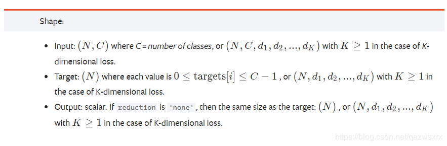
显然，其中N=4, C=31, d1=d2=256, 故target中的1是多余的，是报错的原因。

loss = criterion(logit, torch.squeeze(target).long())

将target变为[4, 256, 256]即可。

CUDNN_STATUS_NOT_SUPPORTED. This error may appear if you passed in a non-contiguous input.

这个问题折腾了我一天，最后竟然是pytorch版本的问题。

pytorch1.4报这个bug， 1.3完美运行

这种莫名其妙找不到原因的bug太让人头疼了，以后决定稳定使用pytorch1.3

!pip install torch===1.3.0 torchvision==0.4.1
!pip3 install 'pillow<7.0.0'

内存泄漏

Further to what it is already mentioned, cycle() and zip() might create a memory leakage problem - especially when using image datasets! To solve that, instead of iterating like this:

dataloaders1 = DataLoader(DummyDataset(0, 100), batch_size=10, shuffle=True)
dataloaders2 = DataLoader(DummyDataset(0, 200), batch_size=10, shuffle=True)
num_epochs = 10

for epoch in range(num_epochs):

    for i, (data1, data2) in enumerate(zip(cycle(dataloaders1), dataloaders2)):

        do_cool_things()

you could use:

dataloaders1 = DataLoader(DummyDataset(0, 100), batch_size=10, shuffle=True)
dataloaders2 = DataLoader(DummyDataset(0, 200), batch_size=10, shuffle=True)
num_epochs = 10

for epoch in range(num_epochs):
    dataloader_iterator = iter(dataloaders1)

    for i, data1 in enumerate(dataloaders2)):

        try:
            data2 = next(dataloader_iterator)
        except StopIteration:
            dataloader_iterator = iter(dataloaders1)
            data2 = next(dataloader_iterator)

        do_cool_things()

Tcl_AsyncDelete: async handler deleted by the wrong thread

matplotlib.pyplot在运行的时候，是需要在主线程(Main Thread)上运行的，然而，我在使用多线程的时候，将使用matplotlib.pyplot的函数用在了子线程里面。之后也在matplotlib的官方FAQ找到了相应的原因，如下图：

解决方法：

将原本的import matplotlib.pyplot as plt修改成以下：

import matplotlib
matplotlib.use('Agg')
from matplotlib import pyplot as plt

lengths’ argument should be a 1D CPU int64 tensor, but got 1D cuda:0 Long tensor

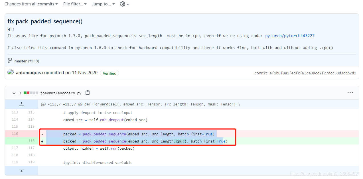
参考https://github.com/joeynmt/joeynmt/pull/119/commits/ef1b0f081fedfcf83ce39cd2f27dcc33d3cbb2d1以及https://github.com/pytorch/pytorch/releases

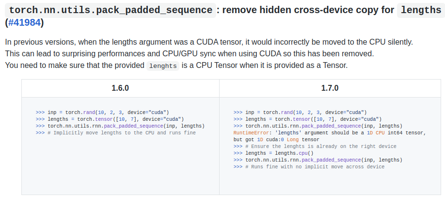
nn.Upsample 和 F.interpolate 无法复现问题

Pytorch 中的 interpolate 是 non-deterministic 的函数，目前没有解决办法。

Setting the seed gives different results each time the code is run #8

CUDA initialization: CUDA unknown error - this may be due to an incorrectly set up environment

> sudo rmmod nvidia_uvm
> sudo modprobe nvidia_uvm

Pytorch模块化功能

Self-Attention

class Self_Attn(nn.Module):
    def __init__(self, in_dim):
        super(Self_Attn, self).__init__()
        self.channel_in = in_dim

        self.query_conv = nn.Conv2d(in_channels=in_dim, out_channels=in_dim//8, kernel_size=1)
        self.key_conv = nn.Conv2d(in_channels=in_dim, out_channels=in_dim//8, kernel_size=1)
        self.value_conv = nn.Conv2d(in_channels=in_dim, out_channels=in_dim, kernel_size=1)
        self.gamma = nn.Parameter(torch.zeros(1))

        self.softmax = nn.Softmax(dim=-1)

    def forward(self, x):
        '''
            inputs: 
                x : input feature maps(B x C x W x H)
            returns:
                out: self attention value + input feature
                attention: B x N x N(N is Width*Height)
        '''
        m_batchsize, C, width, height = x.size()
        proj_query = self.query_conv(x).view(m_batchsize, -1, width*height).permute(0, 2, 1) # B x N x C
        proj_key = self.key_conv(x).view(m_batchsize, -1, width*height) # B x C x N
        energy = torch.bmm(proj_query, proj_key) # batch矩阵的乘法
        # dim=-1， 对列做softmax
        # B x N x N
        attention = self.softmax(energy)
        proj_value = self.value_conv(x).view(m_batchsize, -1, width*height) # B x C x N

        out = torch.bmm(proj_value, attention.permute(0, 2, 1))
        out = out.view(m_batchsize, C, width, height)

        out = self.gamma*out + x
        return out

Spectral Normalization

def l2Normalize(v, eps=1e-12):
    return v / (v.norm() + eps)



class SpectralNorm(nn.Module):
    def __init__(self, module, name='weight', power_iterations=1):
        super(SpectralNorm, self).__init__()
        self.module = module
        self.name = name
        self.power_iterations = power_iterations
        if not self._made_params():
            self._make_params()

    def _update_u_v(self):
        u = getattr(self.module, self.name + "_u")
        v = getattr(self.module, self.name + "_v")
        w = getattr(self.module, self.name + "_bar")

        height = w.data.shape[0]
        for _ in range(self.power_iterations):
            # w: width, hegiht
            # u: height, 1
            v.data = l2Normalize(torch.mv(torch.t(w.view(height, -1).data), u.data))
            # w: height width
            # v: width, 1
            u.data = l2Normalize(torch.mv(w.view(height, -1).data, v.data))

            # w: height, width
            # v: width, 1
            # u: height, 1
            # 内积就相当于转置再乘了， 小技巧get
            sigma = u.dot(w.view(height, -1).mv(v))
            setattr(self.module, self.name, w / sigma.expand_as(w))

    def _made_params(self):
        try:
            u = getattr(self.module, self.name + "_u")
            v = getattr(self.module, self.name + "_v")
            w = getattr(self.module, self.name + "_bar")
            return True
        except AttributeError:
            return False

    
    def _make_params(self):
        w = getattr(self.module, self.name)

        height = w.data.shape[0]
        width = w.view(height, -1).data.shape[1]

        u = nn.Parameter(w.data.new(height).normal_(0, 1), requires_grad=False)
        v = nn.Parameter(w.data.new(width).normal_(0, 1), requires_grad=False)
        u.data = l2Normalize(u.data)
        v.data = l2Normalize(v.data)
        w_bar = nn.Parameter(w.data)

        del self.module._parameters[self.name]

        self.module.register_parameter(self.name + "_u", u)
        self.module.register_parameter(self.name + "_v", v)
        self.module.register_parameter(self.name + "_bar", w_bar)

    def forward(self, *args):
        self._update_u_v()
        return self.module.forward(*args)

Equalized Learning Rate

Pytorch Tricks

释放显存占用

torch.cuda.empty_cache()

查看是否有梯度回传

for name, parms in model.named_parameters():
	print('-->name:', name, '-->grad_requirs:', parms.requires_grad, '--weight', torch.mean(parms.data), ' -->grad_value:', torch.mean(parms.grad))

Tensor与各种图像格式的相互转化

PIL与Tensor

import torch
from PIL import Image
import matplotlib.pyplot as plt

# loader使用torchvision中自带的transforms函数
loader = transforms.Compose([
    transforms.ToTensor()])  

unloader = transforms.ToPILImage()

PIL读取图片转化为Tensor

# 输入图片地址
# 返回tensor变量
def image_loader(image_name):
    image = Image.open(image_name).convert('RGB')
    image = loader(image).unsqueeze(0)
    return image.to(device, torch.float)
	

将PIL图片转化为Tensor

# 输入PIL格式图片
# 返回tensor变量
def PIL_to_tensor(image):
    image = loader(image).unsqueeze(0)
    return image.to(device, torch.float)
	

Tensor转化为PIL图片

# 输入tensor变量
# 输出PIL格式图片
def tensor_to_PIL(tensor):
    image = tensor.cpu().clone()
    image = image.squeeze(0)
    image = unloader(image)
    return image

直接展示tensor格式图片

def imshow(tensor, title=None):
    image = tensor.cpu().clone()  # we clone the tensor to not do changes on it
    image = image.squeeze(0)  # remove the fake batch dimension
    image = unloader(image)
    plt.imshow(image)
    if title is not None:
        plt.title(title)
    plt.pause(0.001)  # pause a bit so that plots are updated

直接保存tensor格式图片

def save_image(tensor, epoch):
    image = tensor.cpu().clone()  # we clone the tensor to not do changes on it
    image = image.squeeze(0)  # remove the fake batch dimension
    image = unloader(image)
    image.save('save_pic/epoch_%d.png'%epoch)

numpy与Tensor

import cv2
import torch
import matplotlib.pyplot as plt

numpy转化为tensor

def toTensor(img):
    assert type(img) == np.ndarray,'the img type is {}, but ndarry expected'.format(type(img))
    img = cv2.cvtColor(img, cv2.COLOR_BGR2RGB)
    img = torch.from_numpy(img.transpose((2, 0, 1)))
    return img.float().div(255).unsqueeze(0)  # 255也可以改为256

tensor转化为numpy

def tensor_to_np(tensor):
    img = tensor.mul(255).byte()
    img = img.cpu().squeeze(0).numpy().transpose((1, 2, 0))
    return img

展示numpy格式图片

def show_from_cv(img, title=None):
    img = cv2.cvtColor(img, cv2.COLOR_BGR2RGB)
    plt.figure()
    plt.imshow(img)
    if title is not None:
        plt.title(title)
    plt.pause(0.001)

展示tensor格式图片

def show_from_tensor(tensor, title=None):
    img = tensor.clone()
    img = tensor_to_np(img)
    plt.figure()
    plt.imshow(img)
    if title is not None:
        plt.title(title)
    plt.pause(0.001)

利用Hook机制获取中间特征

Hook for Tensors

import torch

x = torch.Tensor([0, 1, 2, 3]).requires_grad_()
y = torch.Tensor([4, 5, 6, 7]).requires_grad_()
w = torch.Tensor([1, 2, 3, 4]).requires_grad_()
z = x+y

# ===================
def hook_fn(grad):
    print(grad)

z.register_hook(hook_fn)
# ===================

o = w.matmul(z)

print('=====Start backprop=====')
o.backward()
print('=====End backprop=====')

print('x.grad:', x.grad)
print('y.grad:', y.grad)
print('w.grad:', w.grad)
print('z.grad:', z.grad)

运行结果如下：
=====Start backprop=====
tensor([2., 4., 6., 8.])
=====End backprop=====
x.grad: tensor([2., 4., 6., 8.])
y.grad: tensor([2., 4., 6., 8.])
w.grad: tensor([ 4., 6., 8., 10.])
z.grad: None

对于中间变量z，hook 的使用方式为：z.register_hook(hook_fn)，其中 hook_fn为一个用户自定义的函数，其签名为：

hook_fn(grad) -> Tensor or None

它的输入为变量 z 的梯度，输出为一个 Tensor 或者是 None （None 一般用于直接打印梯度）。反向传播时，梯度传播到变量 z，再继续向前传播之前，将会传入 hook_fn。如果 hook_fn的返回值是 None，那么梯度将不改变，继续向前传播，如果 hook_fn的返回值是 Tensor 类型，则该 Tensor 将取代 z 原有的梯度，向前传播。

Hook for Modules

register forward hook

register_forward_hook的作用是获取前向传播过程中，各个网络模块的输入和输出。对于模块 module，其使用方式为：module.register_forward_hook(hook_fn) 。其中 hook_fn的签名为：

hook_fn(module, input, output) -> None

它的输入变量分别为：模块，模块的输入，模块的输出，和对 Tensor 的 hook 不同，forward hook 不返回任何值，也就是说不能用它来修改输入或者输出的值（注意：从 pytorch 1.2.0 开始，forward hook 也有返回值了，可以修改网络模块的输出），但借助这个 hook，我们可以方便地用预训练的神经网络提取特征，而不用改变预训练网络的结构。下面提供一段示例代码：

import torch
from torch import nn

# 首先我们定义一个模型
class Model(nn.Module):
    def __init__(self):
        super(Model, self).__init__()
        self.fc1 = nn.Linear(3, 4)
        self.relu1 = nn.ReLU()
        self.fc2 = nn.Linear(4, 1)
        self.initialize()
    
    # 为了方便验证，我们将指定特殊的weight和bias
    def initialize(self):
        with torch.no_grad():
            self.fc1.weight = torch.nn.Parameter(
                torch.Tensor([[1., 2., 3.],
                              [-4., -5., -6.],
                              [7., 8., 9.],
                              [-10., -11., -12.]]))

            self.fc1.bias = torch.nn.Parameter(torch.Tensor([1.0, 2.0, 3.0, 4.0]))
            self.fc2.weight = torch.nn.Parameter(torch.Tensor([[1.0, 2.0, 3.0, 4.0]]))
            self.fc2.bias = torch.nn.Parameter(torch.Tensor([1.0]))

    def forward(self, x):
        o = self.fc1(x)
        o = self.relu1(o)
        o = self.fc2(o)
        return o

# 全局变量，用于存储中间层的 feature
total_feat_out = []
total_feat_in = []

# 定义 forward hook function
def hook_fn_forward(module, input, output):
    print(module) # 用于区分模块
    print('input', input) # 首先打印出来
    print('output', output)
    total_feat_out.append(output) # 然后分别存入全局 list 中
    total_feat_in.append(input)


model = Model()

modules = model.named_children() # 
for name, module in modules:
    module.register_forward_hook(hook_fn_forward)

# 注意下面代码中 x 的维度，对于linear module，输入一定是大于等于二维的
# （第一维是 batch size）。在 forward hook 中看不出来，但是 backward hook 中，
# 得到的梯度完全不对。
# 有一篇 hook 的教程就是这里出了错，作者还强行解释

x = torch.Tensor([[1.0, 1.0, 1.0]]).requires_grad_() 
o = model(x)
o.backward()

print('==========Saved inputs and outputs==========')
for idx in range(len(total_feat_in)):
    print('input: ', total_feat_in[idx])
    print('output: ', total_feat_out[idx])

运行结果为：
Linear(in_features=3, out_features=4, bias=True)
input (tensor([[1., 1., 1.]], requires_grad=True),)
output tensor([[ 7., -13., 27., -29.]], grad_fn=<AddmmBackward>)
ReLU()
input (tensor([[ 7., -13., 27., -29.]], grad_fn=<AddmmBackward>),)
output tensor([[ 7., 0., 27., 0.]], grad_fn=<ThresholdBackward0>)
Linear(in_features=4, out_features=1, bias=True)
input (tensor([[ 7., 0., 27., 0.]], grad_fn=<ThresholdBackward0>),)
output tensor([[89.]], grad_fn=<AddmmBackward>)
==========Saved inputs and outputs==========
input: (tensor([[1., 1., 1.]], requires_grad=True),)
output: tensor([[ 7., -13., 27., -29.]], grad_fn=<AddmmBackward>)
input: (tensor([[ 7., -13., 27., -29.]], grad_fn=<AddmmBackward>),)
output: tensor([[ 7., 0., 27., 0.]], grad_fn=<ThresholdBackward0>)
input: (tensor([[ 7., 0., 27., 0.]], grad_fn=<ThresholdBackward0>),)
output: tensor([[89.]], grad_fn=<AddmmBackward>)

register backward hook

和 register_forward_hook相似，register_backward_hook 的作用是获取神经网络反向传播过程中，各个模块输入端和输出端的梯度值。对于模块 module，其使用方式为：module.register_backward_hook(hook_fn) 。其中hook_fn的函数签名为：

hook_fn(module, grad_input, grad_output) -> Tensor or None

它的输入变量分别为：模块，模块输入端的梯度，模块输出端的梯度。需要注意的是，这里的输入端和输出端，是站在前向传播的角度的，而不是反向传播的角度。例如线性模块：o=W*x+b，其输入端为 W，x 和 b，输出端为 o。

如果模块有多个输入或者输出的话，grad_input和grad_output可以是 tuple 类型。对于线性模块：o=W*x+b ，它的输入端包括了W、x 和 b 三部分，因此 grad_input 就是一个包含三个元素的 tuple。

这里注意和 forward hook 的不同：

在 forward hook 中，input 是 x，而不包括 W 和 b。
返回 Tensor 或者 None，backward hook 函数不能直接改变它的输入变量，但是可以返回新的 grad_input，反向传播到它上一个模块。

下面看示例代码：

import torch
from torch import nn


class Model(nn.Module):
    def __init__(self):
        super(Model, self).__init__()
        self.fc1 = nn.Linear(3, 4)
        self.relu1 = nn.ReLU()
        self.fc2 = nn.Linear(4, 1)
        self.initialize()

    def initialize(self):
        with torch.no_grad():
            self.fc1.weight = torch.nn.Parameter(
                torch.Tensor([[1., 2., 3.],
                              [-4., -5., -6.],
                              [7., 8., 9.],
                              [-10., -11., -12.]]))

            self.fc1.bias = torch.nn.Parameter(torch.Tensor([1.0, 2.0, 3.0, 4.0]))
            self.fc2.weight = torch.nn.Parameter(torch.Tensor([[1.0, 2.0, 3.0, 4.0]]))
            self.fc2.bias = torch.nn.Parameter(torch.Tensor([1.0]))

    def forward(self, x):
        o = self.fc1(x)
        o = self.relu1(o)
        o = self.fc2(o)
        return o


total_grad_out = []
total_grad_in = []


def hook_fn_backward(module, grad_input, grad_output):
    print(module) # 为了区分模块
    # 为了符合反向传播的顺序，我们先打印 grad_output
    print('grad_output', grad_output) 
    # 再打印 grad_input
    print('grad_input', grad_input)
    # 保存到全局变量
    total_grad_in.append(grad_input)
    total_grad_out.append(grad_output)


model = Model()

modules = model.named_children()
for name, module in modules:
    module.register_backward_hook(hook_fn_backward)

# 这里的 requires_grad 很重要，如果不加，backward hook
# 执行到第一层，对 x 的导数将为 None，某英文博客作者这里疏忽了
# 此外再强调一遍 x 的维度，一定不能写成 torch.Tensor([1.0, 1.0, 1.0]).requires_grad_()
# 否则 backward hook 会出问题。
x = torch.Tensor([[1.0, 1.0, 1.0]]).requires_grad_()
o = model(x)
o.backward()

print('==========Saved inputs and outputs==========')
for idx in range(len(total_grad_in)):
    print('grad output: ', total_grad_out[idx])
    print('grad input: ', total_grad_in[idx])

运行后的输出为：

Linear(in_features=4, out_features=1, bias=True)
grad_output (tensor([[1.]]),)
grad_input (tensor([1.]), tensor([[1., 2., 3., 4.]]), tensor([[ 7.],
        [ 0.],
        [27.],
        [ 0.]]))
ReLU()
grad_output (tensor([[1., 2., 3., 4.]]),)
grad_input (tensor([[1., 0., 3., 0.]]),)
Linear(in_features=3, out_features=4, bias=True)
grad_output (tensor([[1., 0., 3., 0.]]),)
grad_input (tensor([1., 0., 3., 0.]), tensor([[22., 26., 30.]]), tensor([[1., 0., 3., 0.],
        [1., 0., 3., 0.],
        [1., 0., 3., 0.]]))
==========Saved inputs and outputs==========
grad output:  (tensor([[1.]]),)
grad input:  (tensor([1.]), tensor([[1., 2., 3., 4.]]), tensor([[ 7.],
        [ 0.],
        [27.],
        [ 0.]]))
grad output:  (tensor([[1., 2., 3., 4.]]),)
grad input:  (tensor([[1., 0., 3., 0.]]),)
grad output:  (tensor([[1., 0., 3., 0.]]),)
grad input:  (tensor([1., 0., 3., 0.]), tensor([[22., 26., 30.]]), tensor([[1., 0., 3., 0.],
        [1., 0., 3., 0.],
        [1., 0., 3., 0.]]))

注意事项

register_backward_hook只能操作简单模块，而不能操作包含多个子模块的复杂模块。如果对复杂模块用了 backward hook，那么我们只能得到该模块最后一次简单操作的梯度信息。对于上面的代码稍作修改，不再遍历各个子模块，而是把 model 整体绑在一个 hook_fn_backward上：

model = Model()
model.register_backward_hook(hook_fn_backward) 

输出结果如下：

Model(
  (fc1): Linear(in_features=3, out_features=4, bias=True)
  (relu1): ReLU()
  (fc2): Linear(in_features=4, out_features=1, bias=True)
)
grad_output (tensor([[1.]]),)
grad_input (tensor([1.]), tensor([[1., 2., 3., 4.]]), tensor([[ 7.],
        [ 0.],
        [27.],
        [ 0.]]))
==========Saved inputs and outputs==========
grad output:  (tensor([[1.]]),)
grad input:  (tensor([1.]), tensor([[1., 2., 3., 4.]]), tensor([[ 7.],
        [ 0.],
        [27.],
        [ 0.]]))

我们发现，程序只输出了 fc2 的梯度信息。

除此之外，有人还总结（吐槽）了 backward hook 在全连接层和卷积层表现不一致的地方（Feedback about PyTorch register_backward_hook · Issue #12331 · pytorch/pytorch）

形状
- 在卷积层中，weight 的梯度和 weight 的形状相同
- 在全连接层中，weight 的梯度的形状是 weight 形状的转秩（观察上文中代码的输出可以验证）
grad_input tuple 中各梯度的顺序
- 在卷积层中，bias 的梯度位于tuple 的末尾：grad_input = (对feature的导数，对权重 W 的导数，对 bias 的导数)
- 在全连接层中，bias 的梯度位于 tuple 的开头：grad_input=(对 bias 的导数，对 feature 的导数，对 W 的导数)
当 batchsize>1时，对 bias 的梯度处理不同
- 在卷积层，对 bias 的梯度为整个 batch 的数据在 bias 上的梯度之和：grad_input = (对feature的导数，对权重 W 的导数，对 bias 的导数)
- 在全连接层，对 bias 的梯度是分开的，bach 中每条数据，对应一个 bias 的梯度：grad_input = ((data1 对 bias 的导数，data2 对 bias 的导数 …)，对 feature 的导数，对 W 的导数)

例子

import torch
from torchvision.models import resnet18
import torch.nn as nn
from torchvision import transforms

import matplotlib.pyplot as plt

from numpy import sqrt


def viz(module, input, output):
    # input是个tuple，tuple里是个tensor
    # output是个tensor
    x = output[0][0].cpu()
    # 最多显示4张图
    min_num = np.minimum(4, x.size()[0])
    for i in range(min_num):
        plt.subplot(1, 4, i+1)
        plt.imshow(x[i])
    plt.show()


import cv2
import numpy as np
def main():
    t = transforms.Compose([transforms.ToPILImage(),
                            transforms.Resize((224, 224)),
                            transforms.ToTensor(),
                            transforms.Normalize(mean=[0.485, 0.456, 0.406],
                                                 std=[0.229, 0.224, 0.225])
                            ])

    device = torch.device("cuda:0" if torch.cuda.is_available() else "cpu")

    model = resnet18(pretrained=True).to(device)
    for name, m in model.named_modules():
        # if not isinstance(m, torch.nn.ModuleList) and \
        #         not isinstance(m, torch.nn.Sequential) and \
        #         type(m) in torch.nn.__dict__.values():
        # 这里只对卷积层的feature map进行显示
        if isinstance(m, torch.nn.Conv2d):
            m.register_forward_hook(viz)
    img = cv2.imread(r'D:\Jupyter\GAN-zoo\SEAN\068012.jpg')
    img = t(img).unsqueeze(0).to(device)
    with torch.no_grad():
        model(img)

if __name__ == '__main__':
    main()

绘图

曲线图

import torch

import pandas as pd
import numpy as np 

import seaborn as sns
import matplotlib.pyplot as plt

state = torch.load("./models/state.pth")

df1 = pd.DataFrame(state['rec_loss'], columns=['rec_loss'])
df2 = pd.DataFrame(state['enc_loss'], columns=['enc_loss'])
df3 = pd.DataFrame(state['g_loss'], columns=['g_loss'])
df4 = pd.DataFrame(state['d_loss'], columns=['d_loss'])

f=plt.figure()

f.add_subplot(221)

sns.lineplot(data=df1)

f.add_subplot(222)
sns.lineplot(data=df2)

f.add_subplot(223)
sns.lineplot(data=df3)

f.add_subplot(224)
sns.lineplot(data=df4)


plt.show()

losses

On this page

Torch

torch.add

torch.scatter

torch.cat

torch.reshape

PyTorch view和reshape的区别

torch.max

torch.maximum

torch.argmax

torch.min

torch.minimum

torch.sum

torch.squeeze

torch.chunk

torch.arange

torch.clamp

torch.clip

torch.var

torch.empty

torch.rand

产生噪声的方式

torch.norm

torch.mul 和 torch.matmul

torch.bmm

torch.bmm和torch.matmul的区别

torch.mv

torch.eq

torch.dot

torch.flip

torch.t

torch.numel

torch.full

torch.nonzero

torch.save与torch.load

保存

加载

torch.cuda()

torch.repeat_interleave

torch.argsort

torch.topk

torch.where

借助 torch.where 找到矩阵中指定的数

Tensor

resize

expand

expand_as

repeat

permute

new

masked_fill

torch.distributions

torch.distributions.beta.Beta

torch.backends.cudnn

torch.flatten

torch.meshgrid

torch.einsum

torch.tril

torch.addmm

torch.gather

torch.multinomial

torch.randperm

Pytorch查看版本信息及NVDIA查看版本信息

Torch.nn

torch.nn.Conv2d

torch.nn.Softmax

torch.nn.L1Loss

torch.nn.CrossEntropyLoss

torch.nn.BCELoss

torch.nn.BatchNorm2d

torch.nn.InstanceNorm2d

torch.nn.ReflectionPad2d

torch.nn.MaxPool2d

torch.nn.AvgPool2d

torch.nn.AvgPool3d

nn.ConvTranspose2d与nn.Upsample的区别

nn.PReLU

ModuleList和Sequential

nn.Sequential

nn.ModuleList