On this page
Overview
Description
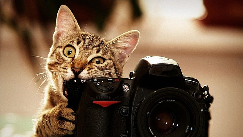
一图胜千言。你知道吗,一张照片可以拯救千万条生命?世界各地每天都有数百万流浪动物在街头受苦或在收容所被安乐死。你可能会认为带着迷人照片的宠物会引起更多的兴趣,并更快地被收养。但怎样才能拍出好照片呢?在数据科学的帮助下,你可以准确地判断宠物照片的吸引力,甚至提出改进建议,让这些被救助的动物有更高的机会拥有爱的家。
PetFinder.my使用基本的可爱指数(Cuteness Meter)来对宠物照片进行排名。它分析了图片组成和其他因素,并将其与成千上万的宠物档案的表现进行了比较。虽然这个基本工具很有用,但它仍处于实验阶段,算法还可以改进。
在本次比赛中,您将分析原始图像和元数据,以预测宠物照片的Pawpularity。你将会在 PetFinder.my 上千个宠物档案中训练和测试你的模型。获胜的版本将会提供更准确的推荐, 这会帮助到动物福利。如果成功,你的解决方案将被应用到人工智能工具中,指导世界各地的庇护所和救援人员提高他们宠物档案的吸引力,自动提高照片质量,并推荐改进构图。因此,流浪狗和流浪猫可以更快地找到它们“永远”的家。在Kaggle社区的一点点帮助下,许多宝贵的生命可以被拯救,更多的幸福家庭可以建立起来。
顶级参与者可能会被邀请合作实施他们的解决方案,并利用他们的人工智能技能创造性地改善全球动物福利。
Evaluation
Root Mean Squared Error 𝑅𝑀𝑆𝐸
提交使用均方根损失打分。 RMSE 定义为:
\[RMSE = \sqrt{\frac{1}{n} \sum_{i=1}^n(y_i - \hat y_i)^2}\]对于每个样本 $i$, 其中 $\hat y_i$ 是预测值, $y_i$ 是原始值
Submission File
对于测试集中的每个 Id, 你必须预测目标变量中 Pawpularity 的概率。 该文件应该包含一个 header ,并具有以下格式:
Id, Pawpularity
0008dbfb52aa1dc6ee51ee02adf13537, 99.24
0014a7b528f1682f0cf3b73a991c17a0, 61.71
0019c1388dfcd30ac8b112fb4250c251, 6.23
00307b779c82716b240a24f028b0031b, 9.43
00320c6dd5b4223c62a9670110d47911, 70.89
etc.
Code Requirements
参赛作品必须通过 Notebooks 提交。为了使“提交”按钮在提交后处于活动状态,必须满足以下条件:
- CPU Notebook <= 9 小时运行时间
- GPU Notebook <= 9 小时运行时间
- 互联网接入禁用
- 允许免费和公开的外部数据,包括预训练的模型
- 提交文件必须命名为
submission.csv
Data
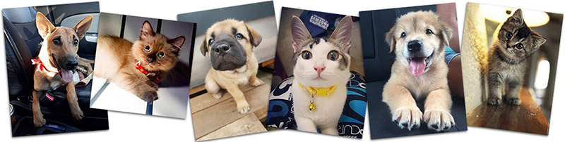
在这个比赛中,你的任务是根据宠物的照片和宠物的文件预测其互动程度。您将会被提供每张照片手工标记的元数据。因此,本次竞赛的数据集包括图像和表格数据。
How Pawpularity Score Is Derived
- Pawpularity Score是通过对不同页面、平台(网页和手机)和各种指标的流量数据进行标准化的算法,从列表页面上的每个宠物的页面视图统计数据中得到的。
- 重复点击、爬虫机器人访问和 sponsored profiles 将从分析中排除。
Purpose of Photo Metadata
- 我们已经包括可选的照片元数据,手动标记每一张照片的关键视觉质量和组成参数。
- 这些标签不是用来推导我们的Pawpularity分数的,但它可能有助于更好地理解内容,并将它们与照片的吸引力联系起来。我们的最终目标是部署人工智能解决方案,可以生成智能建议(如显示更近的宠物正面脸,添加配件,增加主题聚焦等)和自动增强(如亮度,对比度)的照片,所以我们希望有更容易解释的预测。
- 您可以根据自己的需要使用这些标签,还可以选择构建一个中间/补充模型,以根据照片预测标签。如果你的补充模型好,我们也可以把它整合到我们的人工智能工具中。
- 在我们的生产系统中,动态评分的新照片将不包含任何照片标签。如果Pawpularity预测模型需要照片标签分数,我们将使用一个中间模型来推导这些参数,然后再将它们输入最终模型。
Training Data
- train/ -包含 训练图像 {id}.jpg 的文件夹
- train.csv - 元数据(如下所述)为训练集中的每一张照片以及目标,照片的Pawpularity分数。Id列 给出了与照片的文件名相对应的照片唯一的Pet Profile Id。
Example Test Data
除了训练数据,我们还包括一些随机生成的示例测试数据,以帮助您编写提交代码。当你提交的笔记被记分时,这个例子数据将被实际的测试数据(包括提交的样本)所取代。
- test/ - 文件夹中包含与训练集照片类似的格式的随机生成的图像。实际测试数据包含约6800张与训练集照片类似的宠物照片。
- test.csv - 随机生成的元数据类似于训练集元数据。
- sample_submission.csv - 正确格式的样例提交文件。
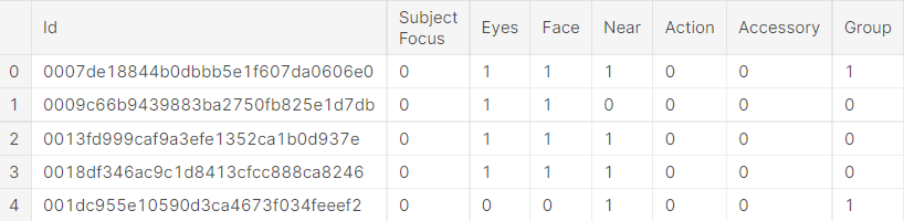
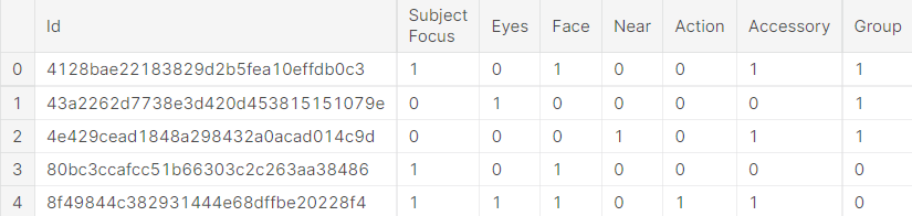
Photo Metadata
在训练集和测试集中 train.csv 和 test.csv 文件分别包含照片的元数据。每一张宠物照片都用1(是)或0(否)的值标记以下每一个特征:
- Focus - 宠物在整洁的背景下显得很突出,不太近/远。
- Eyes - 双眼面向前方或近前方,至少有一只眼睛/瞳孔清晰。
- Face - 相当清晰的脸,正面或近正面。
- Near - 单只宠物占据照片的很大一部分(大约超过50%的照片宽度或高度)。
- Action - 宠物在中间做一个动作(如跳跃)。
- Accessory - 佩戴实物或数字配件/道具(即玩具、数字贴纸),不包括项圈和皮带。
- Group - 照片里不止一只宠物。
- Collage - 数码修饰照片(即数码相框,多张照片的组合)。
- Human - 照片中是否有人。
- Occlusion - 特定的不受欢迎的物体阻塞宠物的部分(例如人,笼子或栅栏)。注意,并非所有阻塞对象都被认为是遮挡。
- Info - 自定义添加的文本或标签(如宠物名,描述)。
- Blur - 特别是宠物的眼睛和脸,焦距明显不清或有噪音。对于模糊条目,Eyes列总是设置为0。
Pawpular : EDA + Understanding + Effnet + W&B
Libraries
%%sh
pip install -q pytorch-lightning==1.1.8
pip install -q timm
pip install -q albumentations
pip install -q --upgrade wandb
import gc
import os
import glob
import sys
import cv2
import imageio
import joblib
import math
import random
import wandb
import math

import numpy as np
import pandas as pd

from scipy.stats import kstest

import matplotlib.pyplot as plt
import matplotlib.patches as patches
from statsmodels.graphics.gofplots import qqplot

plt.rcParams.update({'font.size': 18})
plt.style.use('fivethirtyeight')

import seaborn as sns
import matplotlib

from termcolor import colored

from multiprocessing import cpu_count
from tqdm.notebook import tqdm
from sklearn.model_selection import StratifiedKFold
from scipy.stats import pearsonr

import timm
import torch
import transformers
import torch.nn as nn
import torch.nn.functional as F
from torch.utils.data import DataLoader, Dataset

from sklearn.model_selection import StratifiedKFold
from sklearn.metrics import r2_score, mean_squared_error

import pytorch_lightning as pl
from pytorch_lightning.loggers import WandbLogger
from pytorch_lightning.callbacks import ModelCheckpoint

from albumentations import (
    HorizontalFlip, VerticalFlip, IAAPerspective, ShiftScaleRotate, CLAHE, RandomRotate90,
    Transpose, ShiftScaleRotate, Blur, OpticalDistortion, GridDistortion, HueSaturationValue,
    IAAAdditiveGaussianNoise, GaussNoise, MotionBlur, MedianBlur, IAAPiecewiseAffine, RandomResizedCrop,
    IAASharpen, IAAEmboss, RandomBrightnessContrast, Flip, OneOf, Compose, Normalize, Cutout, CoarseDropout, ShiftScaleRotate, CenterCrop, Resize
)
from albumentations.pytorch import ToTensorV2

import warnings
warnings.simplefilter('ignore')

# Activate pandas progress apply bar
tqdm.pandas()
# Wandb Login
import wandb
wandb.login()
wandb: You can find your API key in your browser here: https://wandb.ai/authorize
wandb: Appending key for api.wandb.ai to your netrc file: /root/.netrc
True
Weights and Biases

Weights & Biases 是让开发人员更快地建立更好的模型的机器学习平台。
您可以使用W&B的轻量级、可互操作的工具:
- 快速跟踪实验
- 版本和数据集上进行迭代
- 评估模型性能
- 复现模型
- 可视化结果与 spot regressions
- 并与同事分享结果
在5分钟内建立W&B,然后在您的机器学习 pipeline 上快速迭代,确保您的数据集和模型在可靠的记录系统中被跟踪和版本化。
在这个笔记本中,我将使用 Weights & Biases 的惊人功能来无缝地执行奇妙的可视化和记录。
Global Config
class config:
    DIRECTORY_PATH = "../input/petfinder-pawpularity-score"
    TRAIN_CSV_PATH = DIRECTORY_PATH + "/train.csv"
    TEST_CSV_PATH = DIRECTORY_PATH + "/test.csv"

    SEED = 42

Config = dict(
    NFOLDS = 5,
    EPOCHS = 1,
    LR = 2e-4,
    IMG_SIZE = (224, 224),
    MODEL_NAME = 'tf_efficientnet_b6_ns',
    DR_RATE = 0.35,
    NUM_LABELS = 1,
    TRAIN_BS = 32,
    VALID_BS = 16,
    min_lr = 1e-6,
    T_max = 20,
    T_0 = 25,
    NUM_WORKERS = 4,
    infra = "Kaggle",
    competition = 'petfinder',
    _wandb_kernel = 'neuracort',
    wandb = False
)
# wandb config
WANDB_CONFIG = {
     'competition': 'PetFinder',
              '_wandb_kernel': 'neuracort'
    }
wandb_logger = WandbLogger(project='pytorchlightning', group='vision', job_type='train',
                           anonymous='allow', config=Config)
def set_seed(seed=config.SEED):
    random.seed(seed)
    os.environ["PYTHONHASHSEED"] = str(seed)
    np.random.seed(seed)

    torch.manual_seed(seed)
    torch.cuda.manual_seed(seed)
    torch.cuda.manual_seed_all(seed)
    torch.backends.cudnn.deterministic = True
    torch.backends.cudnn.benchmark = False

set_seed()
Load Datasets
# Efficient Data Types
dtype = {
    'Id': 'string',
    'Subject Focus': np.uint8, 'Eyes': np.uint8, 'Face': np.uint8, 'Near': np.uint8,
    'Action': np.uint8, 'Accessory': np.uint8, 'Group': np.uint8, 'Collage': np.uint8,
    'Human': np.uint8, 'Occlusion': np.uint8, 'Info': np.uint8, 'Blur': np.uint8,
    'Pawpularity': np.uint8,
}

train = pd.read_csv(config.TRAIN_CSV_PATH, dtype=dtype)
test = pd.read_csv(config.TEST_CSV_PATH, dtype=dtype)
Tabular Exploration
Train Head
train.head()
Test Head
test.head()
Train Info
train.info()
<class 'pandas.core.frame.DataFrame'>
RangeIndex: 9912 entries, 0 to 9911
Data columns (total 14 columns):
 #   Column         Non-Null Count  Dtype
---  ------         --------------  -----
 0   Id             9912 non-null   string
 1   Subject Focus  9912 non-null   uint8
 2   Eyes           9912 non-null   uint8
 3   Face           9912 non-null   uint8
 4   Near           9912 non-null   uint8
 5   Action         9912 non-null   uint8
 6   Accessory      9912 non-null   uint8
 7   Group          9912 non-null   uint8
 8   Collage        9912 non-null   uint8
 9   Human          9912 non-null   uint8
 10  Occlusion      9912 non-null   uint8
 11  Info           9912 non-null   uint8
 12  Blur           9912 non-null   uint8
 13  Pawpularity    9912 non-null   uint8
dtypes: string(1), uint8(13)
memory usage: 203.4 KB
Test Info
test.info()
<class 'pandas.core.frame.DataFrame'>
RangeIndex: 8 entries, 0 to 7
Data columns (total 13 columns):
 #   Column         Non-Null Count  Dtype
---  ------         --------------  -----
 0   Id             8 non-null      string
 1   Subject Focus  8 non-null      uint8
 2   Eyes           8 non-null      uint8
 3   Face           8 non-null      uint8
 4   Near           8 non-null      uint8
 5   Action         8 non-null      uint8
 6   Accessory      8 non-null      uint8
 7   Group          8 non-null      uint8
 8   Collage        8 non-null      uint8
 9   Human          8 non-null      uint8
 10  Occlusion      8 non-null      uint8
 11  Info           8 non-null      uint8
 12  Blur           8 non-null      uint8
dtypes: string(1), uint8(12)
memory usage: 288.0 bytes
Dataset Size
print(f"Training Dataset Shape: {colored(train.shape, 'yellow')}")
print(f"Test Dataset Shape: {colored(test.shape, 'yellow')}")
Training Dataset Shape: (9912, 14)
Test Dataset Shape: (8, 13)
Distribution Plots
# Add File path to Train
def get_image_file_path(image_id):
    return f'/kaggle/input/petfinder-pawpularity-score/train/{image_id}.jpg'

train['file_path'] = train['Id'].apply(get_image_file_path)
widths = []
heights = []
ratios = []
for file_path in tqdm(train['file_path']):
    image = imageio.imread(file_path)
    h, w, _ = image.shape
    heights.append(h)
    widths.append(w)
    ratios.append(w / h)
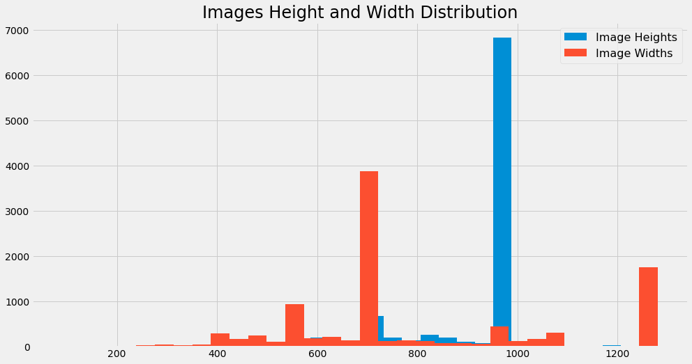
Images Height and Width Distribution
# Images Height and Width Distribution
print(colored('Width Statistics', 'yellow'))
display(pd.Series(widths).describe())
print()

print(colored('Height Statistics', 'yellow'))
display(pd.Series(heights).describe())
print()

plt.figure(figsize=(15,8))
plt.title(f'Images Height and Width Distribution', size=24)
plt.hist(heights, bins=32, label='Image Heights')
plt.hist(widths, bins=32, label='Image Widths')
plt.legend(prop={'size': 16})
plt.show()
Width Statistics
count    9912.000000
mean      804.426251
std       270.211921
min        90.000000
25%       675.000000
50%       720.000000
75%       960.000000
max      1280.000000
dtype: float64
Height Statistics
count    9912.000000
mean      904.284302
std       156.905980
min       113.000000
25%       908.750000
50%       960.000000
75%       960.000000
max      1280.000000
dtype: float64
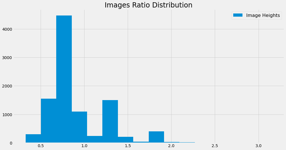
Images Ratio Distribution
# Images Ratio Distribution
print(colored('Ratio Statistics', 'yellow'))
display(pd.Series(ratios).describe())
print()

plt.figure(figsize=(15,8))
plt.title(f'Images Ratio Distribution', size=24)
plt.hist(ratios, bins=16, label='Image Heights')
plt.legend(prop={'size': 16})
plt.show()
Ratio Statistics
count    9912.000000
mean        0.909855
std         0.337773
min         0.326042
25%         0.750000
50%         0.750000
75%         1.038329
max         3.152709
dtype: float64
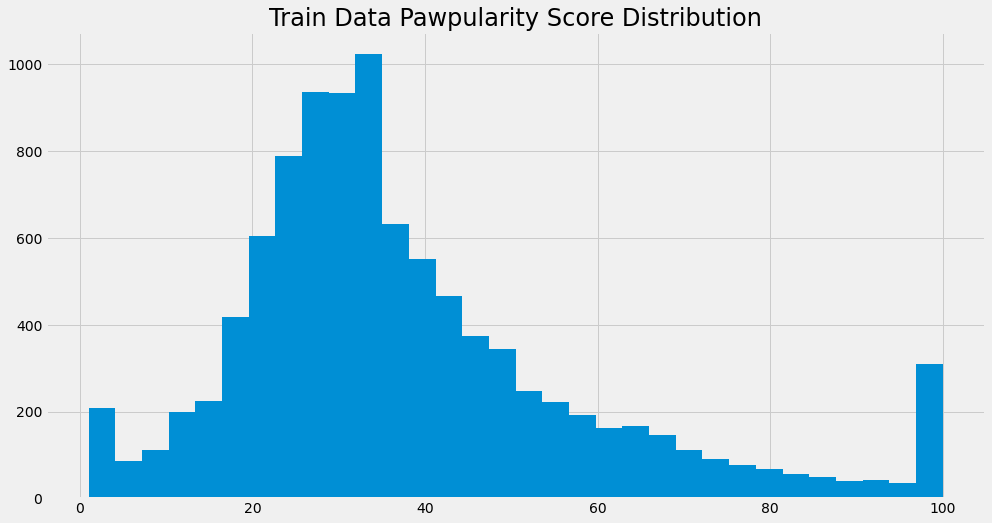
Pawpularity Score Distribution
# Pawpularity Score Distribution
print(colored('Pawpularity Statistics', 'yellow'))
display(train['Pawpularity'].describe())
print()

plt.figure(figsize=(15,8))
plt.title('Train Data Pawpularity Score Distribution', size=24)
plt.hist(train['Pawpularity'], bins=32)
plt.show()
Pawpularity Statistics
count    9912.000000
mean       38.039044
std        20.591990
min         1.000000
25%        25.000000
50%        33.000000
75%        46.000000
max       100.000000
Name: Pawpularity, dtype: float64
Quantile-Quantile plot of Pawpularity distribution
fig = plt.figure()
qqplot(train['Pawpularity'], line='s')
plt.title('Quantile-Quantile plot of Pawpularity distribution',
          fontsize=20, fontweight='bold')
plt.show()
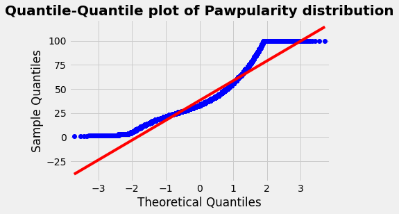
我们注意到这个 QQPlot 的 deviation ,它表明这似乎不是一个高斯分布。我们将使用Kolmogorov-Smirnov测试进行检查(Shapiro-Wilks不适用于大于5000个条目的数据集)。
# Kolmogorov-Smirnov test with Scipy
stat, p = kstest(train['Pawpularity'],'norm')
print('Statistics=%.3f, p=%.3f' % (stat, p))
# interpret
alpha = 0.05
if p > alpha:
    print(f'Sample looks Gaussian (fail to reject H0 at {int(alpha*100)}% test level)')
else:
    print(f'Sample does not look Gaussian (reject H0 at {int(alpha*100)}% test level)')
Statistics=0.990, p=0.000
Sample does not look Gaussian (reject H0 at 5% test level)
测试清楚地表明,该分布不遵循高斯定律。因此,根据所选择的建模对数据进行规范化是很重要的。
Feature Wise Analysis
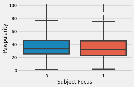
Subject Focus
sns.boxplot(data=train, x='Subject Focus', y='Pawpularity')
plt.show()
sns.histplot(train, x="Pawpularity", hue="Subject Focus", kde=True)
plt.show()

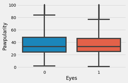
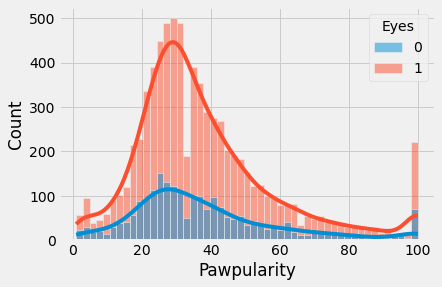
Eyes
sns.boxplot(data=train, x='Eyes', y='Pawpularity')
plt.show()
sns.histplot(train, x="Pawpularity", hue="Eyes", kde=True)
plt.show()
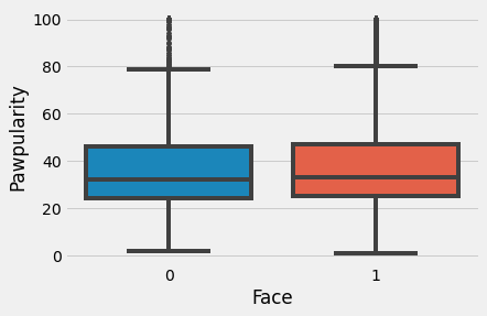
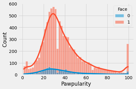
Face
sns.boxplot(data=train, x='Face', y='Pawpularity')
plt.show()
sns.histplot(train, x="Pawpularity", hue="Face", kde=True)
plt.show()
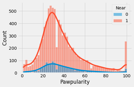
Near
sns.boxplot(data=train, x='Near', y='Pawpularity')
plt.show()
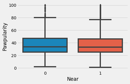
sns.histplot(train, x="Pawpularity", hue="Near", kde=True)
plt.show()
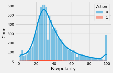
Action
sns.boxplot(data=train, x='Action', y='Pawpularity')
plt.show()
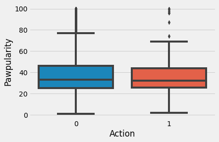
sns.histplot(train, x="Pawpularity", hue="Action", kde=True)
plt.show()
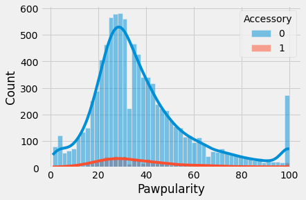
Accessory
sns.boxplot(data=train, x='Accessory', y='Pawpularity')
plt.show()

sns.histplot(train, x="Pawpularity", hue="Accessory", kde=True)
plt.show()
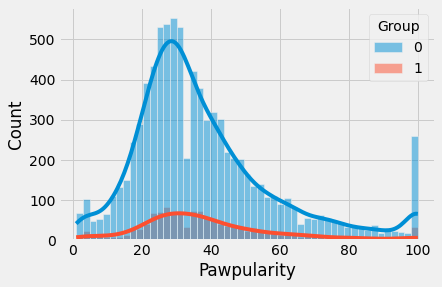
Group
sns.boxplot(data=train, x='Group', y='Pawpularity')
plt.show()
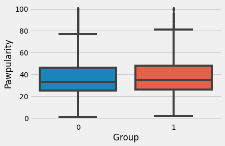
sns.histplot(train, x="Pawpularity", hue="Group", kde=True)
plt.show()
Collage
sns.boxplot(data=train, x='Collage', y='Pawpularity')
plt.show()
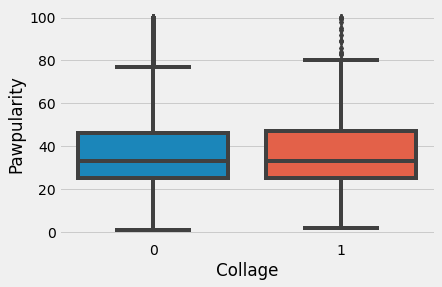
sns.histplot(train, x="Pawpularity", hue="Collage", kde=True)
plt.show()

Human
sns.boxplot(data=train, x='Human', y='Pawpularity')
plt.show()

sns.histplot(train, x="Pawpularity", hue="Human", kde=True)
plt.show()

Occlusion
sns.boxplot(data=train, x='Occlusion', y='Pawpularity')
plt.show()

sns.histplot(train, x="Pawpularity", hue="Occlusion", kde=True)n
plt.show()

Info
sns.boxplot(data=train, x='Info', y='Pawpularity')
plt.show()

sns.histplot(train, x="Pawpularity", hue="Info", kde=True)
plt.show()

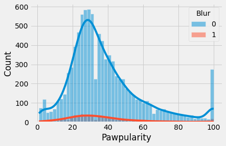
Blur
sns.boxplot(data=train, x='Blur', y='Pawpularity')
plt.show()
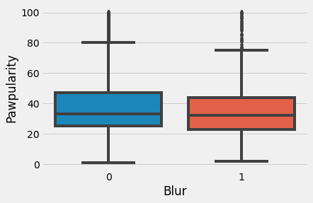
sns.histplot(train, x="Pawpularity", hue="Blur", kde=True)
plt.show()
Pawpularity Score Wise Images
def pawpularity_pics(df, num_images, desired_pawpularity, random_state):

    '''The pawpularity_pics() function accepts 4 parameters: df is a dataframe,
    num_images is the number of images you want displayed, desired_pawpularity
    is the pawpularity score of pics you want to see, and random state ensures reproducibility.'''

    #how many images to display
    num_images = num_images

    #set the rample state for the sampling for reproducibility
    random_state = random_state

    #filter the train_df on the desired_pawpularity and use .sample() to get a sample
    random_sample = df[df["Pawpularity"] == desired_pawpularity].sample(num_images, random_state=random_state).reset_index(drop=True)

    #The for loop goes as many loops as specified by the num_images
    for x in range(num_images):
        #start from the id in the dataframe
        image_path_stem = random_sample.iloc[x]['Id']
        root = '../input/petfinder-pawpularity-score/train/'
        extension = '.jpg'
        image_path = root + str(image_path_stem) + extension

        #get the pawpularity to confirm it worked
        pawpularity_by_id = random_sample.iloc[x]['Pawpularity']

        #use plt.imread() to read in the image file
        image_array = plt.imread(image_path)

        #make a subplot space that is 1 down and num_images across
        plt.subplot(1, num_images, x+1)
        #title is the pawpularity score from the id
        title = pawpularity_by_id
        plt.title(title)
        #turn off gridlines
        plt.axis('off')

        #then plt.imshow() can display it for you
        plt.imshow(image_array)

    plt.show()
    plt.close()
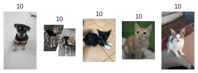
Pawpularity = 10
df = train
num_images = 5
desired_pawpularity = 10
random_state = 1
pawpularity_pics(df, num_images, desired_pawpularity, random_state)
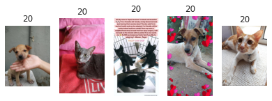
Pawpularity = 20
df = train
num_images = 5
desired_pawpularity = 20
random_state = 1
pawpularity_pics(df, num_images, desired_pawpularity, random_state)
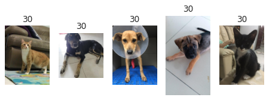
Pawpularity = 30
df = train
num_images = 5
desired_pawpularity = 30
random_state = 1
pawpularity_pics(df, num_images, desired_pawpularity, random_state)
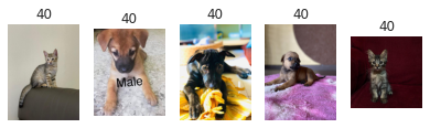
Pawpularity = 40
df = train
num_images = 5
desired_pawpularity = 40
random_state = 1
pawpularity_pics(df, num_images, desired_pawpularity, random_state)
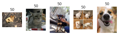
Pawpularity = 50
df = train
num_images = 5
desired_pawpularity = 50
random_state = 1
pawpularity_pics(df, num_images, desired_pawpularity, random_state)
Pawpularity = 60
df = train
num_images = 5
desired_pawpularity = 60
random_state = 1
pawpularity_pics(df, num_images, desired_pawpularity, random_state)
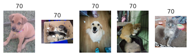
Pawpularity = 70
df = train
num_images = 5
desired_pawpularity = 70
random_state = 1
pawpularity_pics(df, num_images, desired_pawpularity, random_state)
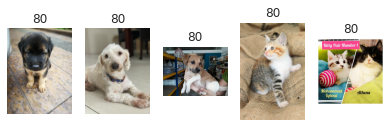
Pawpularity = 80
df = train
num_images = 5
desired_pawpularity = 80
random_state = 1
pawpularity_pics(df, num_images, desired_pawpularity, random_state)
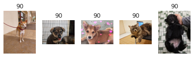
Pawpularity = 90
df = train
num_images = 5
desired_pawpularity = 90
random_state = 1
pawpularity_pics(df, num_images, desired_pawpularity, random_state)
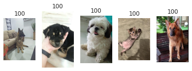
Pawpularity = 100
df = train
num_images = 5
desired_pawpularity = 100
random_state = 1
pawpularity_pics(df, num_images, desired_pawpularity, random_state)
Dataset and Augmentations
Lightning Dataset
class PetfinderData(Dataset):
    def __init__(self, df, is_test=False, augments=None):
        self.df = df
        self.is_test = is_test
        self.augments = augments

        self.images, self.meta_features, self.targets = self._process_df(self.df)

    def __getitem__(self, index):
        img = self.images[index]
        meta_feats = self.meta_features[index]
        meta_feats = torch.tensor(meta_feats, dtype=torch.float32)

        img = cv2.imread(img)
        img = img[:, :, ::-1]
        img = cv2.resize(img, Config['IMG_SIZE'])

        if self.augments:
            img = self.augments(image=img)['image']

        if not self.is_test:
            target = torch.tensor(self.targets[index], dtype=torch.float32)
            return img, meta_feats, target
        else:
            return img, meta_feats

    def __len__(self):
        return len(self.df)

    def _process_df(self, df):
        TRAIN = "../input/petfinder-pawpularity-score/train"
        TEST = "../input/petfinder-pawpularity-score/test"

        if not self.is_test:
            df['Id'] = df['Id'].apply(lambda x: os.path.join(TRAIN, x+".jpg"))
        else:
            df['Id'] = df['Id'].apply(lambda x: os.path.join(TEST, x+".jpg"))

        meta_features = df.drop(['Id', 'Pawpularity'], axis=1).values

        return df['Id'].tolist(), meta_features, df['Pawpularity'].tolist()
Augmentations
class Augments:
    """
    Contains Train, Validation Augments
    """
    train_augments = Compose([
        Resize(*Config['IMG_SIZE'], p=1.0),
        HorizontalFlip(p=0.5),
        VerticalFlip(p=0.5),
        Normalize(
            mean=[0.485, 0.456, 0.406],
            std=[0.229, 0.224, 0.225],
            max_pixel_value=255.0,
            p=1.0
        ),
        ToTensorV2(p=1.0),
    ],p=1.)

    valid_augments = Compose([
        Resize(*Config['IMG_SIZE'], p=1.0),
        Normalize(
            mean=[0.485, 0.456, 0.406],
            std=[0.229, 0.224, 0.225],
            max_pixel_value=255.0,
            p=1.0
        ),
        ToTensorV2(p=1.0),
    ], p=1.)
Efficientnet Model and Understanding
What is Scaling?
Scaling 通常是为了提高模型在特定任务上的准确性,例如ImageNet分类。尽管有时候研究员不太关心模型的 efficient, 因为竞赛是为了击败SOTA, 如果 scaling 做的正确,也可以帮助提高模型的效率。
Types of Scaling for CNNs
对于CNN来说有三种 scaling 维度:
- Depth - 深度指网络的深度,相当于网络的层数。
- Width - 宽度指网络的宽度。 例如,宽度的一种度量是Conv层中的通道数量。
- Resolution - 分辨率是传递给CNN的图像分辨率。
下面的图表(来自论文)将让你清楚地了解在不同维度上缩放的含义。我们也将详细讨论这些问题。
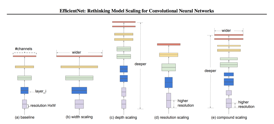
Depth Scaling (d)
通过深度来 Scaling 一个网络是最常见的 Scaling 方式。 深度可以通过分别增加或者删除层数来 Scale up 或者 Scale down。 ResNet 可以从 ResNet-50 Scale up 到 ResNet-200, 也可以从 ResNet-50 scale down 到 ResNet-18。
但是为什么深度 Scaling 呢?直觉告诉我们,更深层次的网络可以捕捉到更丰富、更复杂的特征,并能很好地概括新任务。
很好,让我们把网络增加到1000层呢?如果我们有足够的资源和机会的话, 我们不介意增加更多的层。
说起来容易做起来难! 从理论上讲,随着层数的增加,网络性能会得到改善,但实际情况并非如此。随着我们深入,梯度消失是最常见的问题之一。
即使你避免梯度消失,以及使用一些技术使训练平稳,添加更多的层并不总是有帮助。例如,ResNet-1000与ResNet-101具有相似的精度。
Width Scaling (w)
当我们想要保持模型较小时,这是常用的方法。更宽的网络往往能够捕获更细粒度的特征。而且,更小的模型更容易训练。
现在有什么问题?问题是,即使你可以使你的网络非常宽,用浅模型(较浅但较宽),精度很快会饱和。
Resolution (r)
我们可以直观地说,在高分辨率的图像中,特征更细粒度,因此高分辨率图像应该工作得更好。这也是为什么在像目标检测这样的复杂任务中,我们使用300x300、512x512或600x600的图像分辨率的原因之一。
但这并不是线性的。精度增益下降得很快。例如,将分辨率从500x500提高到560x560并不会产生显著的改进。
以上三点导致了我们的第一个观察结果:放大网络的任何维度(宽度、深度或分辨率)都会提高精度,但对于更大的模型,精度增益会降低。
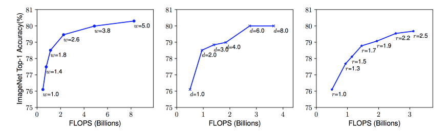
用不同的网络 Width (w)、Depth (d)和 Resolution (r) 系数放大 Baseline 模型。网络的宽度、深度和分辨率越高,网络的精度越高,但精度增益在达到80%后就会迅速饱和,这说明了一维缩放的局限性。
Combined Scaling
是的,我们可以结合不同维度的缩放,研究员们已经提出了一些观点:
- 尽管在二维或三维上 arbitrary scaling 是可能的,但 arbitrary scaling 是一项乏味的任务。
- 大多数情况下,手动 scaling 的精度和效率都不理想。
直觉告诉我们,随着图像分辨率的增加,网络的深度和宽度也应该增加。随着深度的增加,更大的感受野可以捕捉到类似的特征,包括图像中更多的像素。此外,随着宽度的增加,将捕获更多的细粒度特性。为了验证这一直觉,作者对每个维度进行了一系列实验,使用不同的缩放值。例如,如本文下图所示,在同样的FLOPS成本下,宽度缩放的分辨率越高,精度越高。
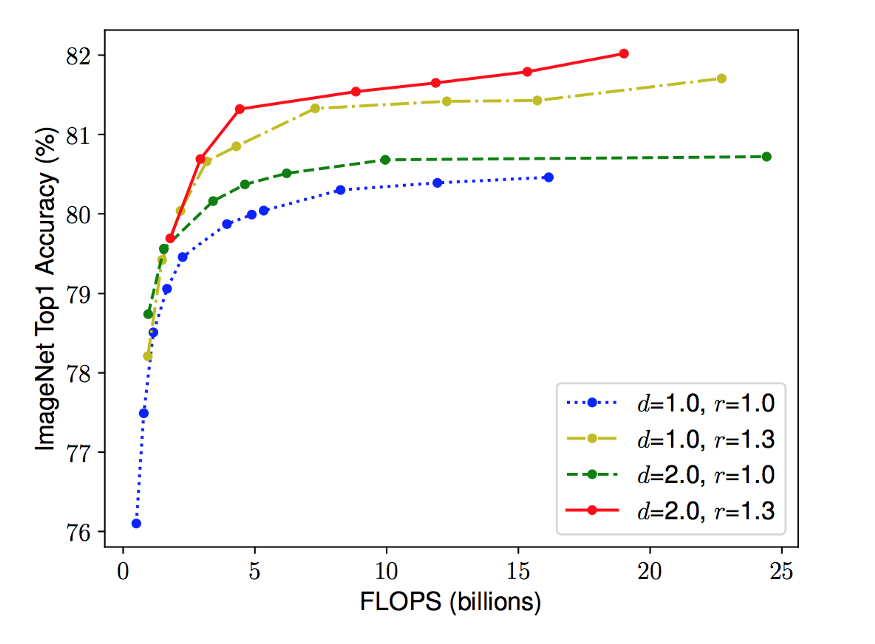
不同基线网络的网络宽度缩放。线中的每个点表示不同宽度系数(w)的模型。所有基线网络均来自表1。第一个基线网络(d=1.0, r=1.0)有18个卷积层,分辨率为224x224,而最后一个基线(d=2.0, r=1.3)有36个卷积层,分辨率为299x299。
这些结果导致了我们的第二个观察: 在 CNN 缩放期间平衡网络的所有维度(宽度、深度和分辨率),以获得更高的准确性和效率是至关重要的。
Proposed Compound Scaling
作者提出了一种简单而有效的缩放技术,即使用复合系数 $\phi$ 来均匀缩放网络的宽度、深度和分辨率:
\[\text{depth} : d = \alpha^\phi \\ \text{width}: w = \beta^{\phi} \\ \text{resolution}: r = \gamma^{\phi} \\ \text{s.t. } \alpha · \beta^2 · \gamma^2 \approx 2 \\ \alpha \geq 1, \beta \geq 1, \gamma \geq 1\]$\phi$ 是一个特定用户的系数, 它控制多少资源可用, $\alpha$ 、 $\beta$ 和 $\gamma$ 指定分别如何分配这些资源给网络的深度、宽度 和 分辨率。
在一个 CNN 中, 卷积层是网络中计算成本最高的地方。 同样,卷积运算的FLOPS是与 $d$, $w^2$, $r^2$ 成比例的, 例如将深度增加一倍将使FLOPS增加一倍,而将宽度或分辨率增加一倍将使FLOPS增加几乎四倍。 因此,为了确保总FLOPS不超过 $2^ \varphi$, 因此增加约束 $(\alpha * \beta^2 * \gamma^2) \approx 2$。
EfficientNet Architecture
缩放不会改变层操作,因此最好先有一个良好的基线网络,然后使用提出的复合缩放沿不同维度缩放它。作者通过神经结构搜索(NAS)获得了他们的基本网络,该搜索优化了准确性和FLOPS。该体系结构与M-NASNet相似,因为它是使用类似的搜索空间找到的。网络的 layers/block 如下所示:
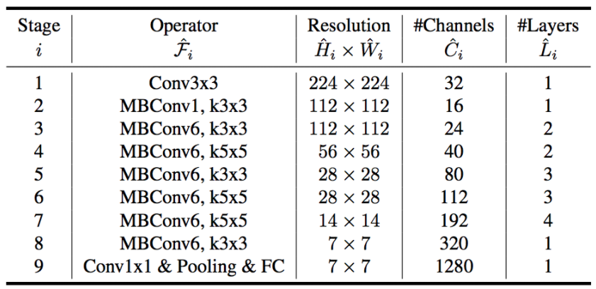
MBConv块没什么特别的,只是一个Inverted Residual Block(在MobileNetV2中使用),有些地方有 Squeeze 和 Excite 块。
现在我们有了基本网络,我们可以为缩放参数寻找最优值。如果我们回顾条件方程,您将很快意识到我们总共有四个参数要搜索 $\alpha$, $\beta$, $\gamma$ 和 $\varphi$。
1) 固定 $\varphi = 1$, 假设可用的资源增加了两倍,然后为 $\alpha$, $\beta$ 和 $\gamma$执行一个小型网格搜索。 对于 baseline 网络 B0, 它表明最优的值为 $\alpha = 1.2$, $\beta = 1.1$ 和 $\gamma = 1.15$, 使得 $\alpha * \beta^2 * \gamma^2 \approx 2$。
2) 现在固定 $\alpha$, $\beta$ 和 $\gamma$ 为常数(上面步骤找到的值) 并且用不同的 $\varphi$ 值实验。 不同的 $\varphi$ 值产生 EfficientNets $B1 - B7$。
class PetFinderModel(pl.LightningModule):
    def __init__(self, pretrained=True):
        super(PetFinderModel, self).__init__()
        self.model = timm.create_model(Config['MODEL_NAME'], pretrained=pretrained)

        self.n_features = self.model.classifier.in_features
        self.model.reset_classifier(0)
        self.fc = nn.Linear(self.n_features + 12, Config['NUM_LABELS'])

        self.train_loss = nn.MSELoss()
        self.valid_loss = nn.MSELoss()

    def forward(self, images, meta):
        features = self.model(images)
        features = torch.cat([features, meta], dim=1)
        output = self.fc(features)
        return output

    def training_step(self, batch, batch_idx):
        imgs = batch[0]
        meta = batch[1]
        target = batch[2]

        out = self(imgs, meta)
        train_loss = torch.sqrt(self.train_loss(out, target))

        logs = {'train_loss': train_loss}

        return {'loss': train_loss, 'log': logs}

    def validation_step(self, batch, batch_idx):
        imgs = batch[0]
        meta = batch[1]
        target = batch[2]

        out = self(imgs, meta)
        valid_loss = torch.sqrt(self.valid_loss(out, target))

        return {'val_loss': valid_loss}

    def validation_end(self, outputs):
        avg_loss = torch.stack([x['val_loss'] for x in outputs]).mean()
        logs = {'val_loss': avg_loss}

        print(f"val_loss: {avg_loss}")
        return {'avg_val_loss': avg_loss, 'log': logs}

    def configure_optimizers(self):
        opt = torch.optim.Adam(self.parameters(), lr=Config['LR'])
        sch = torch.optim.lr_scheduler.CosineAnnealingLR(
            opt,
            T_max=Config['T_max'],
            eta_min=Config['min_lr']
        )

        return [opt], [sch]
Data Folds
# Run the Kfolds training loop
kf = StratifiedKFold(n_splits=Config['NFOLDS'])
train_file = pd.read_csv("../input/petfinder-pawpularity-score/train.csv")

for fold_, (train_idx, valid_idx) in enumerate(kf.split(X=train_file, y=train_file['Pawpularity'])):
    print(f"{'='*20} Fold: {fold_} {'='*20}")

    train_df = train_file.loc[train_idx]
    valid_df = train_file.loc[valid_idx]

    train_set = PetfinderData(
        train_df,
        augments = Augments.train_augments
    )

    valid_set = PetfinderData(
        valid_df,
        augments = Augments.valid_augments
    )

    train = DataLoader(
        train_set,
        batch_size=Config['TRAIN_BS'],
        shuffle=True,
        num_workers=Config['NUM_WORKERS'],
        pin_memory=True
    )
    valid = DataLoader(
        valid_set,
        batch_size=Config['VALID_BS'],
        shuffle=False,
        num_workers=Config['NUM_WORKERS']
    )

    checkpoint_callback = ModelCheckpoint(
        monitor="val_loss",
        dirpath="./",
        filename=f"fold_{fold_}_{Config['MODEL_NAME']}",
        save_top_k=1,
        mode="min",
    )

    model = PetFinderModel()
    trainer = pl.Trainer(
        max_epochs=Config['EPOCHS'],
        gpus=1,
        callbacks=[checkpoint_callback],
        logger= wandb_logger
    )
    trainer.fit(model, train, valid)
CLIP Prompt Feature Engineering | XGB
Introduction
我在这个比赛中的第一个想法是,在预测动物受欢迎程度时,可爱是一个重要因素。这本 notebook 探讨了如何使用CLIP的多模态表示(以及对抽象概念的理解)进行特性工程。
import torch
import torch.nn as nn
from torch.utils.data import Dataset, DataLoader
from pathlib import Path
from os.path import join
import numpy as np
import pandas as pd
import clip, os, skimage
import matplotlib.pyplot as plt
import seaborn as sns
from PIL import Image
from tqdm import tqdm

clip.available_models()
['RN50', 'RN101', 'RN50x4', 'ViT-B/32']
model, preprocess = clip.load("../input/openai-clip/ViT-B-32.pt", jit=False)
model = model.cuda().eval()
input_resolution = model.visual.input_resolution
context_length = model.context_length
vocab_size = model.vocab_size

print("Model parameters:", f"{np.sum([int(np.prod(p.shape)) for p in model.parameters()]):,}")
print("Input resolution:", input_resolution)
print("Context length:", context_length)
print("Vocab size:", vocab_size)
Model parameters: 151,277,313
Input resolution: 224
Context length: 77
Vocab size: 49408
Visualising the Data
train_image_path = Path("../input/petfinder-pawpularity-score/train")
file_names = [f.name for f in train_image_path.iterdir() if f.suffix == ".jpg"]
original_images = []
images = []
plt.figure(figsize=(15, 12))
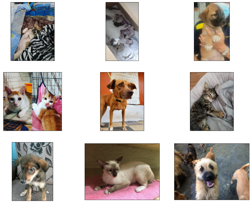
for filename in file_names[:9]:
image = Image.open(join(train_image_path, filename))
plt.subplot(3, 3, len(images) + 1)
plt.imshow(image)
plt.xticks([])
plt.yticks([])
original_images.append(image)
images.append(preprocess(image))
Prompt Feature Engineering
Multimodal Neurons in Artificial Neural Networks 表明 CLIP 能够学习到抽象概念, 例如 emotions 或者 geographical regions。 有了一些关于什么使得动物更受欢迎的先验知识, 这可以创造一些有趣的特征。
有了良好定义的 prompts, 从图像中提取复杂概念是可能的。 我们使用语言和图像嵌入之间的余弦相似度来提取特征进行建模。
texts = ['Cute',
         'Funny',
         'Derp', # let's see if this works
         'Small',
         'Happy',
         'Sad',
         'Aggressive',
         'Friendly',
         'Old',
         'Young',
         'Love']
image_input = torch.tensor(np.stack(images)).cuda()
text_tokens = clip.tokenize(texts).cuda()
with torch.no_grad():
    image_features = model.encode_image(image_input).float()
    text_features = model.encode_text(text_tokens).float()

image_features /= image_features.norm(dim=-1, keepdim=True)
text_features /= text_features.norm(dim=-1, keepdim=True)

similarity_matrix = torch.inner(text_features, image_features).cpu()
count = len(texts)

plt.figure(figsize=(20, 16))
plt.imshow(similarity_matrix, vmin=0.1, vmax=0.3, cmap = 'RdBu')

plt.yticks(range(count), texts, fontsize=18)
plt.xticks([])

for i, image in enumerate(original_images):
    plt.imshow(image, extent=(i - 0.5, i + 0.5, -1.6, -0.6), origin="lower")
for x in range(similarity_matrix.shape[1]):
    for y in range(similarity_matrix.shape[0]):
        plt.text(x, y, f"{similarity_matrix[y, x]:.2f}", ha="center", va="center", size=12)

for side in ["left", "top", "right", "bottom"]:
    plt.gca().spines[side].set_visible(False)

plt.xlim([-0.5, count - 0.5])
plt.ylim([count + 0.5, -2])

plt.title("Cosine similarity matrix between text and image features", size=20, loc='left')
plt.show()
RAPIDS SVR Boost
Boost CV LB +0.2 with RAPIDS SVR Head
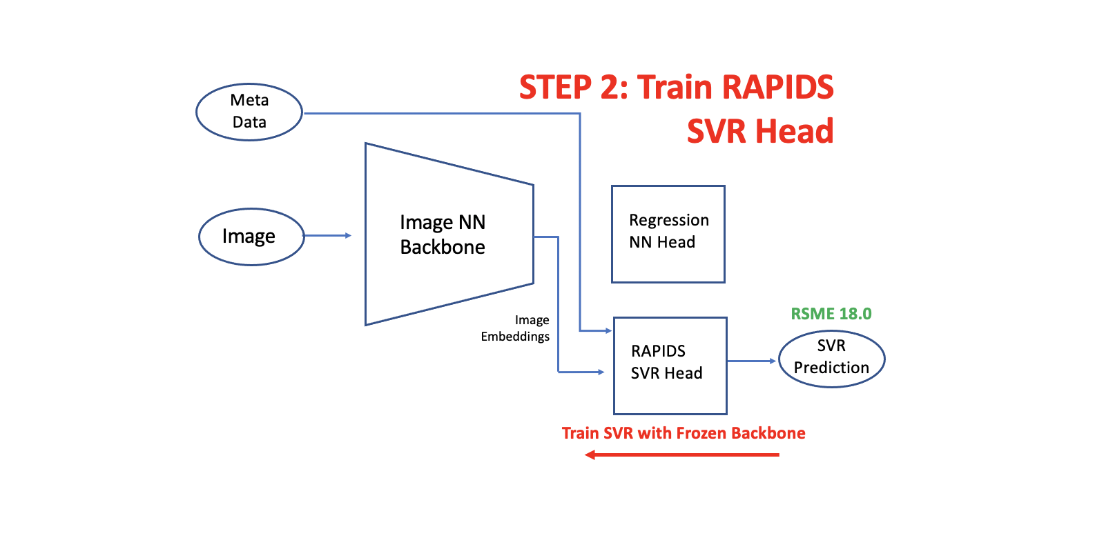
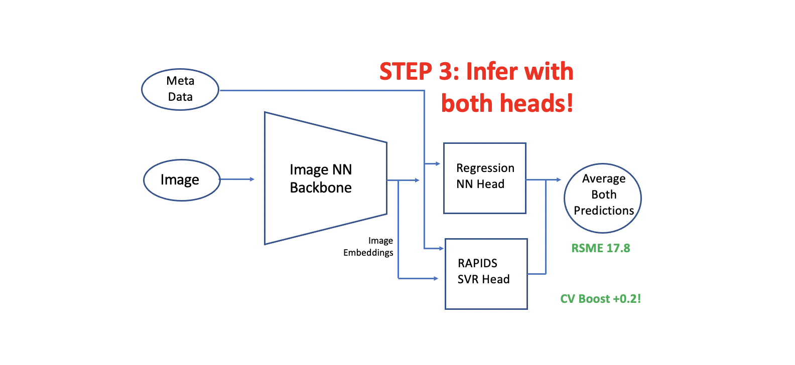
在这个notebook中, 我们展示如何添加一个 PAPIDS SVR 第二个头到一个已经训练好的有第一个头的 CNN 或者 Image Transformer模型中。
我们提取图像嵌入(from the trained fold models) 并且为每个 fold 训练额外的 RAPIDS SVR 头。 原始的NN头取得了CV RSME 18.0 并且 新的 RAPIDS SVR 头取得 CV RSME 18.0。 两个头都非常的多样性因为 NN 头使用 分类(BCE)损失, 而SVR头使用回归损失。 在推理过程中, 我们用两个头预测。 当我们平均两个头的预测时,我们得到了 CV RMSE 17.8。
这里说明的技术可以应用于CV LB boost的任何训练图像(或NLP)模型。 在这个 Notebook 的第一个版本,我们训练SVR头和保存 fold 模型。然后,在后来的 notebook 版本和Kaggle submission 期间,我们加载保存的SVR模型(从这个 notebook 的 version 1,它被制成一个Kaggle数据集)。
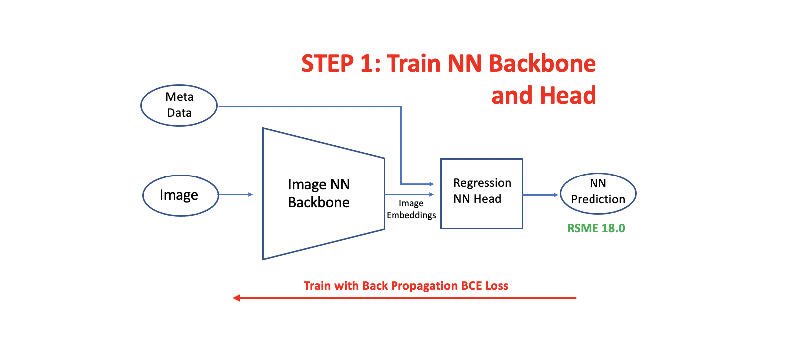
How to Add RAPIDS SVR Head
建立 double head 模型有三个步骤。第一步是训练你的图像神经网络 backbone 和 head。下一步是用从冻结图像神经网络 backbone 中提取的嵌入来训练我们的RAPIDS SVR head。最后,我们用l两个 head 进行推断,并将预测结果平均。
Load Libraries
# based on the post here: https://www.kaggle.com/c/petfinder-pawpularity-score/discussion/275094

import sys
sys.path.append("../input/tez-lib/")
sys.path.append("../input/timmmaster/")

import tez
import albumentations
import pandas as pd
import cv2
import numpy as np
import timm
import torch.nn as nn
from sklearn import metrics
import torch
from tez.callbacks import EarlyStopping
from tqdm import tqdm
import math

class args:
    batch_size = 16
    image_size = 384

def sigmoid(x):
    return 1 / (1 + math.exp(-x))