On this page
Attention Pooling: Nadaraya-Watson Kernel Regression
现在你知道了图10.1.3框架下注意力机制的主要组成部分。 概括地说,queries(volitional cues)和keys(nonvolitional cues)之间的相互作用实现attention pooling。注意力池化选择性地聚集 values (sensory inputs)来产生输出。在本节中,我们将更详细地描述注意力池化,让你从高层次上了解注意力机制在实践中是如何工作的。具体来说,1964年提出的Nadaraya-Watson核回归模型是一个简单而完整的例子,展示了机器学习的注意力机制。
import torch
from torch import nn
from d2l import torch as d2l
Generating the Dataset
为了简单起见,让我们考虑下面的回归问题:给定一个输入输出对的数据集 ${(x_1, y_1), …, (x_n, y_n)}$, 如何学习 $f$ 对 任意的新输入 $x$, 去预测输出 $\hat y = f(x)$?
这里我们根据以下带有噪声项 $\epsilon$ 的非线性函数生成一个人工数据集:
\[y_i = 2\sin(x_i) + x_i^{0.8} + \epsilon \tag{10.2.1}\]其中 $\epsilon$ 服从正态分布,均值为0,标准差为0.5。同时生成50个训练样本和50个测试样本。 为了以后更好地可视化注意力模式,按顺序排好 training input。
n_train = 50
# 采样50个点, 从小到大排列
x_train, _ = torch.sort(torch.rand(n_train) * 5)

def f(x):
    return 2 * torch.sin(x) + x**0.8

y_train = f(x_train) + torch.normal(0.0, 0.5, (n_train,))  # Training outputs
x_test = torch.arange(0, 5, 0.1)  # Testing examples
y_truth = f(x_test)  # Ground-truth outputs for the testing examples
n_test = len(x_test)  # No. of testing examples
n_test
输出:
50
下面的函数绘制了所有训练样本(用圆表示)、生成函数 $f$ 生成的 不含噪声项的 ground-truth数据(用Truth标记)和学习到的预测函数(用Pred标记)。
Average Pooling
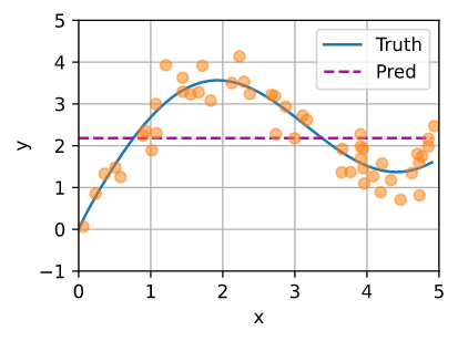
对于这个回归问题, 我们从 “dumbest” 的estimator开始: 用平均池化对所有训练输出进行平均:
\[f(x) = \frac{1}{n} \sum_{i=1}^n y_i\]绘制如下。 如我们所看到的,这个estimator确实没有那么聪明。
y_hat = torch.repeat_interleave(y_train.mean(), n_test)
plot_kernel_reg(y_hat)
Nonparametric Attention Pooling
显然,平均池、池化忽略了输入 $x_i$。 Nadaraya [Nadaraya, 1964] 和 Waston [Watson, 1964]提出了一个更好的想法,根据输入位置对输出 $y_i$ 进行加权:
\[f(x) = \sum_{i=1}^n \frac{K(x - x_i)}{\sum_{j=1}^n K (x - x_j)} y_i \tag{10.2.3}\]其中 $K$ 是 一个 kernel。 (10.2.3) 中的 estimator 叫做 Nadaraya-Watson kernel regression。 这里我们不深入 kernels 的细节。 回想一下图10.1.3中的注意力机制框架。从注意力的角度来看,我们可以将(10.2.3)改写为一种更广义的注意力池化形式:
\[f(x) = \sum_{i=1}^n \alpha(x, x_i)y_i \tag{10.2.4}\]其中 $x$ 是 query 以及 $(x_i, y_i)$ 是 key-value 对。 比较 (10.2.4) 和 (10.2.2), 这里的注意力池化是 values $y_i$ 的 加权平均。 (10.2.4) 中的 注意力权重 $\alpha(x, x_i)$ 根据 $\alpha$ 所建模的 query $x$ 和 key $x_i$ 之间的交互, 分配给对应的 value $y_i$。 对于任何query,它在所有 key-value 对上的注意力权值都是一个有效的概率分布: 它们是非负的,总和为1。
为了获得注意力池化的直观认识,我们可以考虑定义为高斯核:
\[K(\mu) = \frac{1}{\sqrt{2 \pi}} \exp(- \frac{u^2}{2}) \tag{10.2.5}\]将高斯核代入 (10.2.4) 和 (10.2.3):
\[\begin{aligned} f(x) &= \sum_{i=1}^n \alpha(x, x_i) y_i \\ &= \sum_{i=1}^n \frac{\exp(-\frac{1}{2}(x - x_i)^2)}{\sum_{j=1}^n \exp(-\frac{1}{2}(x - x_j)^2)} y_i \\ &= \sum_{i=1}^n softmax (-\frac{1}{2}(x - x_i)^2)y_i \end{aligned} \tag{10.2.6}\]在10.2.6中,给定query $x$ 的 key $x_i$ 将通过赋值给 key 对应的 value $y_i$ 更大的权重 而 获得更多的attention。
值得注意的是,Nadaraya-Watson核回归是一个非参数模型。因此(10.2.6)是非参数注意力池化的一个例子。预测的线是平滑的,比平均池化产生的线更接近 ground-truth。
# Shape of `X_repeat`: (`n_test`, `n_train`), where each row contains the
# same testing inputs (i.e., same queries)
X_repeat = x_test.repeat_interleave(n_train).reshape((-1, n_train))
# Note that `x_train` contains the keys. Shape of `attention_weights`:
# (`n_test`, `n_train`), where each row contains attention weights to be
# assigned among the values (`y_train`) given each query
attention_weights = nn.functional.softmax(-(X_repeat - x_train)**2 / 2, dim=1)
# Each element of `y_hat` is weighted average of values, where weights are
# attention weights
# 每个 Q 对 50 个 K 求权值, 所以乘出来对50个y加权
y_hat = torch.matmul(attention_weights, y_train)
plot_kernel_reg(y_hat)

解释一下这里的代码, 假设 x_test 为 {0, 1, 2,3, 4}, n_train为 3, 那么 x_test.repeat_interleave(n_train)的结果如下图:
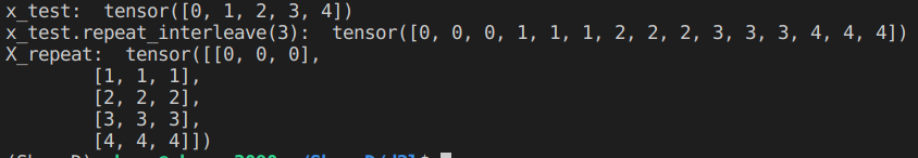
行对应 train, 列对应 test。
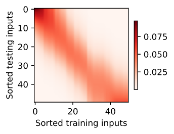
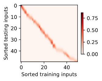
现在让我们来看看注意力权重。在这里 testing inputs 入是 queries,而 training inputs 是 keys。由于两个输入都是排序的,我们可以看到 query-key 对越接近,注意力池化中的注意力权重就越高。
d2l.show_heatmaps(
    attention_weights.unsqueeze(0).unsqueeze(0),
    xlabel='Sorted training inputs', ylabel='Sorted testing inputs')
Parametric Attention Pooling
非参数Nadaraya-Watson核回归具有 consistency 的好处: 只要有足够的数据,这个模型就会收敛到最优解。尽管如此,我们可以很容易地将可学习的参数整合到注意力池化中。
例如,与(10.2.6)稍有不同的是,下面的 query $x$ 与 key $x_i$ 之间的距离 乘以一个可学习的参数 $w$:
\[\begin{aligned} f(x) &= \sum_{i=1}^n \alpha (x, x_i) y_i \\ &= \sum_{i=1}^n \frac{\exp(-\frac{1}{2}((x - x_i)w)^2)}{\sum_{j=1}^n \exp(-\frac{1}{2}((x - x_j)w)^2)}y_i \\ &= \sum_{i=1}^n softmax(-\frac{1}{2} ((x - x_i)w)^2))y_i \end{aligned} \tag{10.2.7}\]在本节的其余部分,我们将通过学习(10.2.7)中的注意力池化参数来训练这个模型。
Batch Matrix Multiplication
为了更有效地计算minibatch的attention,我们可以利用深度学习框架提供的批矩阵乘法工具。
假设第一个 minibatch 包含 $n$ 个形状为 $a \times b$ 的矩阵 $X_1, …, X_n$ , 第二个 minibatch 包含 $n$ 个形状为 $b \times c$ 的矩阵 $Y_1, …, Y_n$。 它们的批矩阵乘法结果是 $n$ 个 形状为 $a \times c$ 的矩阵 $X_1Y_1, …, X_nY_n$。 因此, 给定两个形状为 $(n, a, b)$ 和 $(n, b, c)$ 的tensor, 它们的批矩阵乘法输出为 $(n, a, c)$。
X = torch.ones((2, 1, 4))
Y = torch.ones((2, 4, 6))
torch.bmm(X, Y).shape
torch.Size([2, 1, 6])
在注意机制的背景下,我们可以使用minibatch矩阵乘法来计算minibatch中值的加权平均值。
weights = torch.ones((2, 10)) * 0.1
values = torch.arange(20.0).reshape((2, 10))
torch.bmm(weights.unsqueeze(1), values.unsqueeze(-1))
Defining the Model
下面我们利用minibatch矩阵乘法,基于(10.2.7)中的参数化注意力池化,定义了Nadaraya-Watson核回归的参数化版本。
class NWKernelRegression(nn.Module):
    def __init__(self, **kwargs):
        super().__init__(**kwargs)
        self.w = nn.Parameter(torch.rand((1,), requires_grad=True))

    def forward(self, queries, keys, values):
        # Shape of the output `queries` and `attention_weights`:
        # (no. of queries, no. of key-value pairs)
        #--- dim_0是batch, dim_1是n_train ---
        queries = queries.repeat_interleave(keys.shape[1]).reshape(
            (-1, keys.shape[1]))
        self.attention_weights = nn.functional.softmax(
            -((queries - keys) * self.w)**2 / 2, dim=1)
        # Shape of `values`: (no. of queries, no. of key-value pairs)
        return torch.bmm(self.attention_weights.unsqueeze(1),
                         values.unsqueeze(-1)).reshape(-1)
Training
接下来,我们将训练数据集转换为 key 和 value 来训练注意力模型。在参数化注意力池化中,任何训练输入都要从所有训练样本中取key-value对(除了它自己),以预测它的输出。
怎么训练这个参数呢?就是用一个训练样本去和其他训练样本作attention, 然后算出结果的loss, 反向传播更新参数。
# Shape of `X_tile`: (`n_train`, `n_train`), where each column contains the
# same training inputs
#--- 用于提取 keys ---
X_tile = x_train.repeat((n_train, 1))
# Shape of `Y_tile`: (`n_train`, `n_train`), where each column contains the
# same training outputs
#--- 用于提取 values ---
Y_tile = y_train.repeat((n_train, 1))
# Shape of `keys`: ('n_train', 'n_train' - 1)
keys = X_tile[(1 - torch.eye(n_train)).type(torch.bool)].reshape(
    (n_train, -1))
# Shape of `values`: ('n_train', 'n_train' - 1)
values = Y_tile[(1 - torch.eye(n_train)).type(torch.bool)].reshape(
    (n_train, -1))
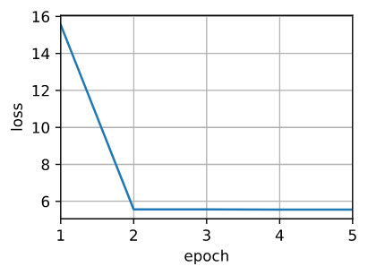
利用平方损失和随机梯度下降对参数化注意力模型进行训练。
net = NWKernelRegression()
loss = nn.MSELoss(reduction='none')
trainer = torch.optim.SGD(net.parameters(), lr=0.5)
animator = d2l.Animator(xlabel='epoch', ylabel='loss', xlim=[1, 5])

for epoch in range(5):
    trainer.zero_grad()
    # Note: L2 Loss = 1/2 * MSE Loss. PyTorch has MSE Loss which is slightly
    # different from MXNet's L2Loss by a factor of 2. Hence we halve the loss
    l = loss(net(x_train, keys, values), y_train) / 2
    l.sum().backward()
    trainer.step()
    print(f'epoch {epoch + 1}, loss {float(l.sum()):.6f}')
    animator.add(epoch + 1, float(l.sum()))
训练参数化注意力模型后,我们可以绘制其预测图。试图用噪声来拟合训练数据集,预测的直线要比先前绘制的非参数数据集平滑得多。
# Shape of `keys`: (`n_test`, `n_train`), where each column contains the same
# training inputs (i.e., same keys)
keys = x_train.repeat((n_test, 1))
# Shape of `value`: (`n_test`, `n_train`)
values = y_train.repeat((n_test, 1))
y_hat = net(x_test, keys, values).unsqueeze(1).detach()
plot_kernel_reg(y_hat)

与非参数的注意力池化相比,在可学习和参数化设置中,具有较大注意力权值的区域变得更清晰。
Summary
- Nadaraya-Watson核回归是一个带有注意力机制的机器学习的例子。
- Nadaraya-Watson核回归的注意力池化是训练输出的加权平均值。从注意的角度来看,注意力权重是根据 query 和 与 value 匹配的 key 分配给值的。
- 注意力池化可以是非参数的,也可以是参数的。
Exercises
- 增加训练样本的数量。你能更好地学习非参数Nadaraya-Watson核回归吗?
- 我们在参数化注意池化实验中 学习到的 $w$ 的价值是什么? 为什么在可视化注意力权重时,它会使权重区域更清晰?
- 我们如何将超参数添加到非参数的Nadaraya-Watson核回归来更好地预测?
- 为本节的核回归设计另一个参数化注意力池化。训练这个新模型,并把它的注意力权重可视化。